Introduction
Accurate and fast access to copper ore grades is crucial for mineral resource exploration, mining, and reserve assessment [1, 2]. After the anomalous or mineral information is obtained using conventional methods, the grade of the mineral deposit must be further confirmed. Core samples obtained from drilling are generally analyzed using chemical methods to determine the mineral grade and chemical element composition [3]. However, this method cannot obtain real-time information on the ore layer location, grade, and other significant details. Analyzing core samples in a laboratory involves relatively complex technical procedures, long waiting times for results, and high costs [4]. In addition, elemental analysis through core sampling has several issues, such as unavoidable sampling errors, time-consuming analytical projects, and inaccurate operational results [5].
The prompt gamma neutron activation analysis (PGNAA) technique employs nuclear reactions between neutrons and samples [6]. Qualitative and quantitative analyses of a sample can be achieved by detecting the energy and intensity of the characteristic gamma rays produced during a nuclear reaction. As a real-time nuclear analysis method, PGNAA technology enables rapid, nondestructive, highly sensitive, and multi-element analyses [7]. It has been applied in coal mining, limestone mining, copper mining, and explosive or chemical weapons detection [8-11].
The process of analyzing spectral information from the collected gamma ray spectrum to determine the relative elemental content is commonly known as inversion or spectral unfolding [12]. Analytical methods for the gamma ray energy spectrum in PGNAA include subtraction, matrix correction, peak area, and least squares methods [13-17]. However, owing to the nonlinear phenomenon in PGNAA [18], the elemental content exhibit a nonlinear relationship with the characteristic peak area. Therefore, the conventional single-peak energy spectrum analysis method is not applicable for the quantitative analysis of PGNAA. Moreover, the full-spectrum analysis method, which involves a large amount of work and a high degree of difficulty, requires the accurate acquisition of spectral libraries for individual elements or compounds [19].
In recent years, the cross application of machine learning and gamma spectral analysis has become increasingly widespread. Machine learning methods for analyzing the gamma energy spectra of PGNAA have attracted much attention [20]. Ghal-Eh et al. applied a neural network approach to analyze the Cl content in aqueous solutions [21]. For the elemental analysis of cement, Peng et al. proposed a back propagation (BP) algorithm to process gamma spectra to obtain the Si, Ca, and Fe contents [22]. Shahabinejad et al. analyzed the Cl and water contents in crude oil using a multilayer perceptron (MLP) model [23].
As an important metallic material, Cu is widely used in electrical engineering, mechanical engineering, and communication technology [24]. Many researchers have employed the PGNAA technique to determine the grade of copper ores. Charbucinski et al. constructed a PGNAA logging device that included a 252Cf neutron source and bismuth germanium oxide (BGO) detector. This device can be used to estimate the Cu grade in the blast holes [25]. To determine the copper–nickel ore grades, Tian et al. proposed a PGNAA formation-logging model in Monte Carlo N-Particle (MCNP) and obtained the grades of copper, nickel, and iron using the least-squares method [26].
In the spectral unfolding process of copper ores, a significant challenge arises because of the similarity between the characteristic Cu and Fe peaks [27]. Therefore, it is important to accurately determine the quantitative effect of Fe on Cu. Conventional spectral analysis methods face challenges in addressing this issue [28]. However, machine-learning methods can establish correlations between gamma-ray spectra and elemental content by constructing neural networks and optimizing weights [29, 30]. This approach effectively addresses the quantitative problems associated with the PGNAA technique for copper-grade analysis.
In this study, a copper-grade analysis method combining the PGNAA technique and vision transformer (ViT) models is proposed. First, a PGNAA model for copper ore measurements is established, and the structural parameters of the model are optimized using the Monte Carlo method. Subsequently, the gamma-ray spectra of copper ores with different grades are obtained using MCNP. These spectra are used for training and testing the machine learning models. Finally, the ViT model is employed to identify the copper ore grade and associated minerals.
Methods and materials
To enable effective mineral grade identification using gamma energy spectrum data, the ViT method was applied in a supervised learning manner. Figure 1 shows the flowchart of the proposed ViT application framework, which comprises three main steps. The first step is the dimension optimization of the PGNAA device structure, the second is ViT modeling for ore-grade identification, and the third is the evaluation of the ViT model.
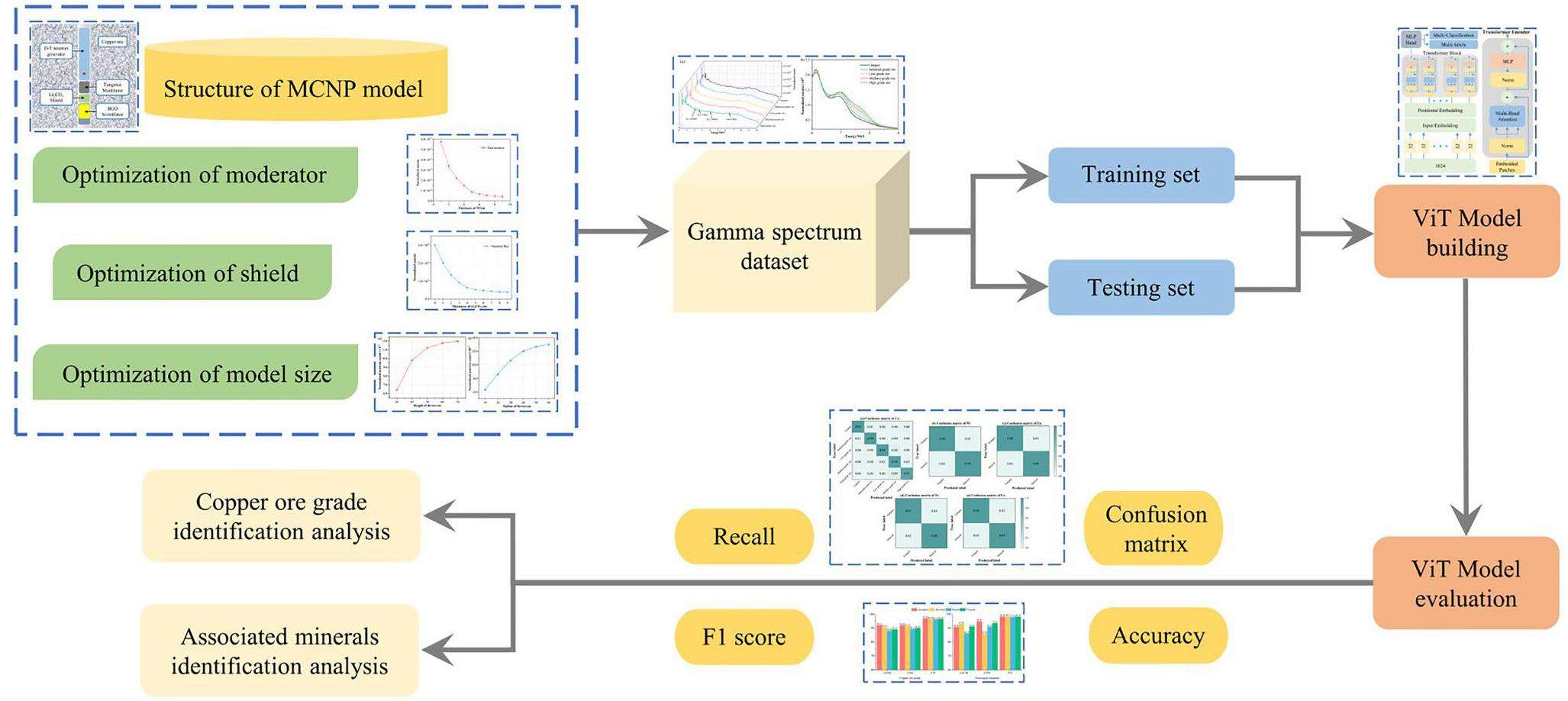
The device structure was optimized using the Monte Carlo method, aiming to determine the optimal thicknesses of the moderator and shield, as well as the device size. Subsequently, the gamma energy spectrum data of copper ores of different grades, simulated using the Monte Carlo method, were preprocessed to construct the input dataset of the model. The hyperparameters of the model were carefully fine-tuned using a grid search method. The performance of the ViT model was evaluated by analyzing the identification results of the copper grade and associated minerals.
Monte Carlo simulation of the PGNAA device
Based on the theory of neutron-gamma distribution, a PGNAA measurement model was established using the Monte Carlo method. As shown in Fig. 2, the model barrel, made of polyethylene, has a cylindrical structure. The PGNAA device was located in the center of the model barrel and consisted of a deuterium tritium (D-T) neutron generator, a BGO detector, and a shielding layer. The dimensions of the neutron generator were 7 cm×70 cm (diameter × height). The BGO crystals had dimensions of 7.62 cm×7.62 cm (diameter × height). To improve the performance of the PGNAA device, parameters including the size of the neutron moderator, the thermal neutron absorption material, and the dimensions of the device must be optimized.
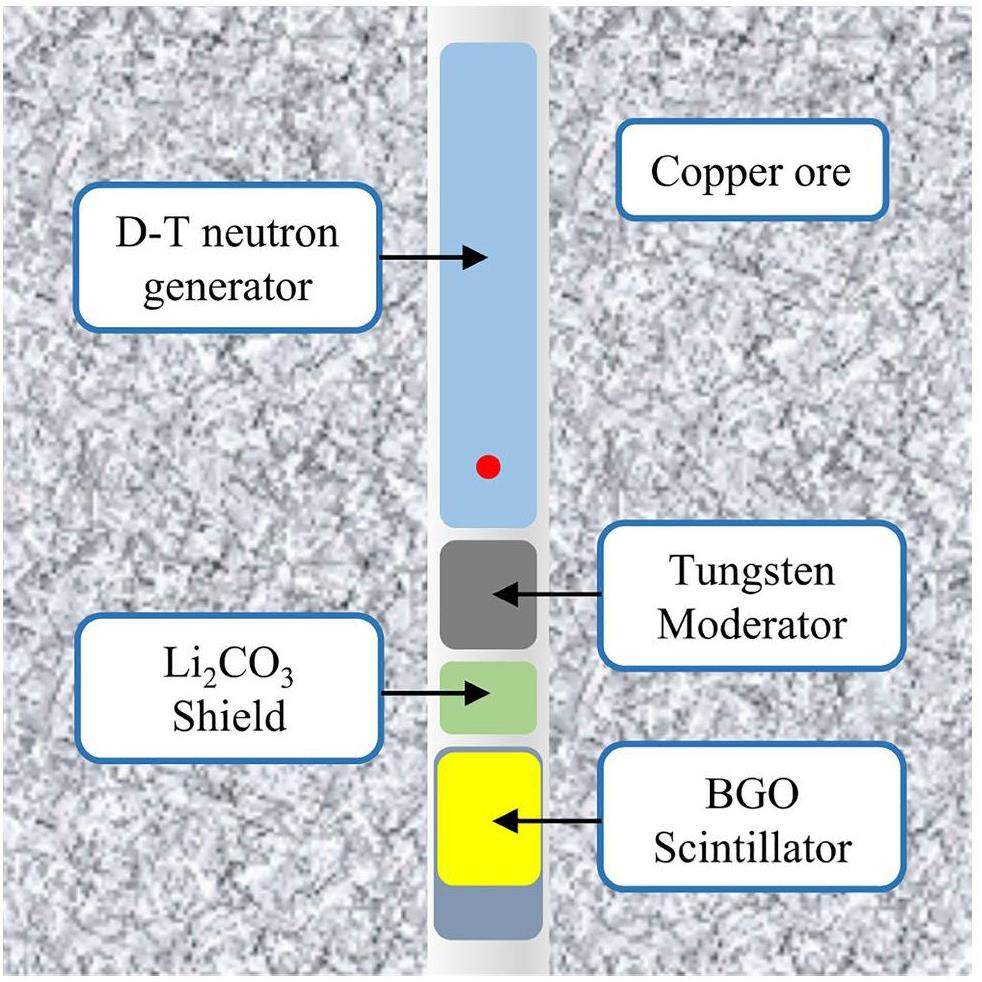
Neutrons entering a gamma detector cause activation noise [31]. To minimize the activation noise, a combination of heavy metals and the Li2CO3 scheme was employed for neutron shielding. Heavy metals were used to thermally decelerate the 14 MeV energy neutrons produced by the D-T neutron generator. Subsequently, thermal neutrons are absorbed by Li2CO3.
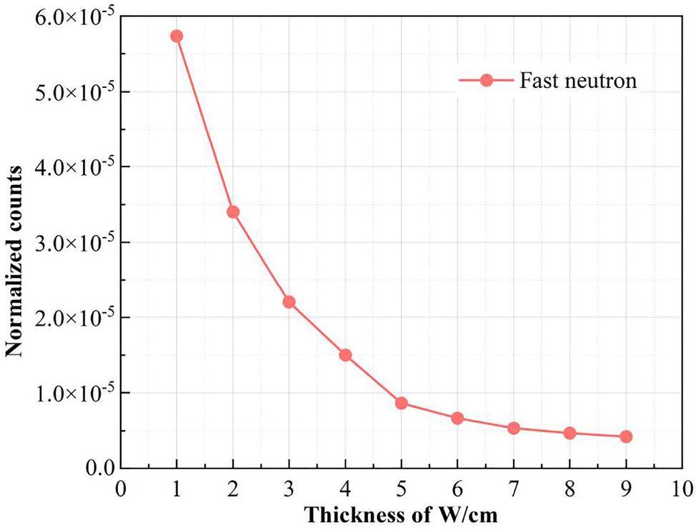
Tungsten is an ideal material for slowing neutrons via inelastic scattering. These reactions can rapidly reduce the neutron energy and slow fast neutrons to thermal neutrons [32, 33]. The fast neutron flux was statistically computed by varying the thickness of tungsten. The decrease in fast neutron flux with increasing tungsten thickness is shown in Fig. 3. When the tungsten thickness reached 7 cm, the shielding effect on fast neutrons reached 90%. Considering the moderating effect and model dimensions, the tungsten thickness was set to 7 cm.
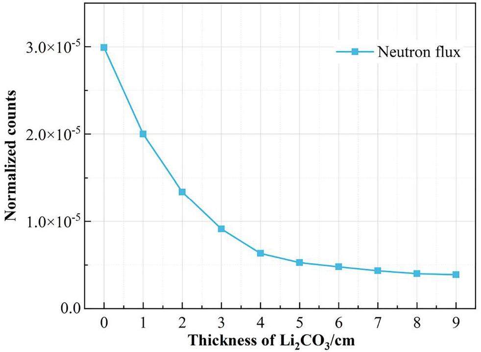
Li2CO3, as a thermal neutron absorption material, was placed between the tungsten and the gamma detector to minimize neutron entry into the gamma detector [34]. The detector neutron fluxes with different Li2CO3 thicknesses were calculated using the F4 card, as shown in Fig. 4. As the Li2CO3 thickness increased, the neutron flux gradually decreased. At a thickness of 5 cm, the neutron flux was significantly reduced. The detector was effectively protected when its thickness was 5 cm. Therefore, an Li2CO3 thickness of 5 cm was used.
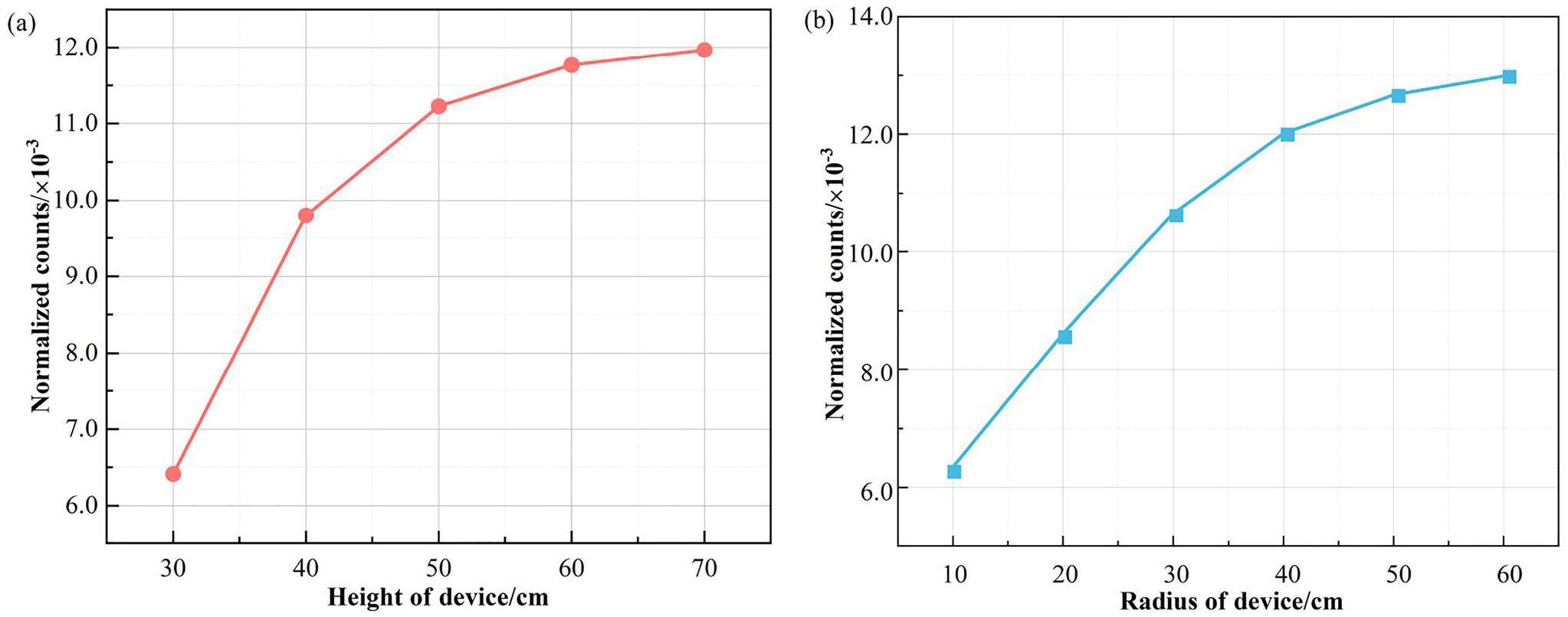
The radius and height of the model barrel were varied to determine the optimal structure. The characteristic peak region of copper in the gamma-ray spectrum ranged from 7.0 MeV to 8.5 MeV. The gamma ray count in this region obtained using the BGO detector verified this result. Based on the simulation, the count of the characteristic peak region of copper increased and then leveled off at approximately 70 cm, as shown in Fig. 5(a). The height of the setup was therefore set to 70 cm. Figure 5(b) shows the relationship between the count of the characteristic peak regions of copper and the radius of the model barrel. The count rapidly increased at first and then became saturated at approximately 50 cm. Therefore, the radius of the setup was set as 50 cm.
ViT model
Transformer models, which represent a neural network architecture based on self-attention mechanisms, have been widely applied to natural language processing (NLP) and other sequence modeling tasks [35]. The ViT model was found to surpass a convolutional neural network (CNN) model on extremely large-scale datasets by entirely replacing the convolutional structure with a transformer structure in classification tasks [36].
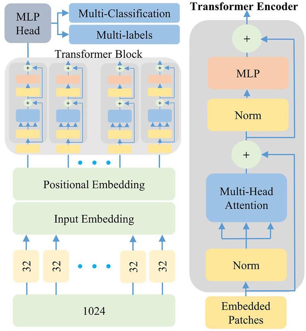
The ViT model structure is illustrated in Fig. 6. A one-dimensional gamma energy spectrum was used as the input dataset for the model. The entire spectrum was divided into 32 segments, where each segment corresponded to positional encoding from 0 to 31 using the tokenization method from NLP. Subsequently, the data were fed into the encoder module for calculation. The encoder consisted of six identical stacked transformer blocks. Each transformer block included a multihead attention mechanism sublayer and a multilayer perceptron sublayer. In the multi-head attention mechanism sub-layer, multiple self-attention mechanism modules were employed in parallel to enhance the attention diversity and improve the expressive capacity of the model. Before the data entered each sublayer, they were normalized to ensure that the mean and variance were relatively stable. This step can accelerate the model training process. When the computation within the sublayer was completed, the residual connections that retain the original input information were employed to directly merge the outputs and inputs of the sublayer. All transformer blocks in the ViT encoder were configured with the same output dimensions. The output of each transformer block was encoded and fed into the MLP classification head, which ultimately resulted in category prediction of the input spectrum.
Hyperparameter tuning
To evaluate the classification performance of the ViT model, two additional classifiers (Long short-term memory (LSTM) and CNN) were built in Python based on the PyTorch library. All three models were trained and tested using the same input dataset. Because the selection of hyperparameters significantly effects the ViT model for grade identification, the hyperparameters must be optimized. A grid search is an effective hyperparameter optimization strategy that can exhaustively search for the optimized hyperparameters of a model. During the grid-search process, a multidimensional grid with successive candidate parameter values was generated, allowing the enumeration of combinations of tunable parameters. Subsequently, the performance metrics of the model were calculated for different parameter combinations. The parameter combination with the best performance metrics was selected as the final model parameter. Table 1 lists the hyperparameter optimization results for each model.
| Model | Parameters | Optimal value |
|---|---|---|
| LSTM | Input_size | 1024 |
| Hidden_size | 256 | |
| Num_layers | 2 | |
| learning_rate | 0.01 | |
| Epoch | 100 | |
| CNN | Conv_layers | 2 |
| Max_pool_layers | 2 | |
| Linear_layers | 2 | |
| Kernel_size | 7 | |
| Number_of_kernels | 3 | |
| Stride | 3 | |
| Learning_rate | 0.001 | |
| Activation_function | tanh | |
| Epoch | 100 | |
| ViT | Patch_size | 32 |
| Num_layers | 6 | |
| Embedding_dim | 512 | |
| Num_heads | 4 | |
| Mlp_dim | 128 | |
| Dropout | 0.1 | |
| Learning_rate | 0.0001 | |
| Num_classes | 5 | |
| Epoch | 100 |
Model evaluation
To compare and determine the best-performing classification model, the input dataset was divided into training and test sets. After training with the training set, the models were evaluated using the test set to determine the number of true positives (TPs), false positives (FPs), true negatives (TNs), and false negatives (FNs). The following evaluation metrics were calculated to measure the performance of the classifier models [37]:
Accuracy refers to the proportion of samples correctly predicted by the model relative to the total number of samples. Accuracy represents the overall predictive accuracy of the classifier for all samples, which can be calculated using Eq. (1).
Dataset
To construct the dataset required for machine learning, the gamma spectrum of copper ore was obtained using MCNP. The material card of the MCNP was set according to the actual copper mineral composition [38]. The primary elements in the Cu ore and their contents are listed in Table 2. In total, 4400 energy spectrum data points were obtained. Based on the copper content, the data were divided into five categories: gangue (0 to 0.2%), industrial-grade copper ore (0.2 to 0.5%), low-grade copper ore (0.5 to 1.5%), medium-grade copper ore (1.5 to 2%), and high-grade copper ore (2 to 3%).
| Element | Cu | Pb | Zn | Fe | Co | Si | Al | O | Ca | K |
|---|---|---|---|---|---|---|---|---|---|---|
| Content (%) | 0–3 | 0–0.6 | 0–1 | 0–10 | 0–0.03 | 25–35 | 8–15 | 40–50 | 3–6 | 1–5 |
Cu is associated with minerals such as pyrite (FeS2), sphalerite (ZnS), galena (PbS), and cobaltite (CoAsS) [39]. Therefore, copper ores often contain associated minerals, such as Pb, Zn, Fe, and Co. Machine-learning models were used to identify the presence of associated minerals in the copper ore. Ores containing Pb, Zn, Fe, and Co below the cut-off grade were designated as gangue, whereas those above the cut-off grade were designated as minerals, based on the content of the associated elements in the ore. The cut-off grades for each associated element are listed in Table 3.
| Component | Pb | Zn | Fe | Co |
|---|---|---|---|---|
| Content (%) | 0.3 | 0.5 | 5 | 0.01 |
Results and Discussion
Gamma spectrum analysis of copper ore
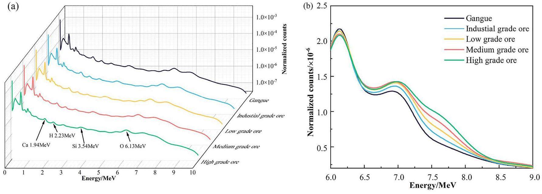
The gamma ray spectra of copper ores with different grades obtained by Monte Carlo simulations are shown in Fig. 7. The energy range was 0–10.0 MeV. Characteristic peaks of major elements such as Ca (1.94 MeV), Si (3.54 MeV), and O (6.13 MeV) were observed. The characteristic peaks of Cu (7.63 MeV and 7.91 MeV) were inconspicuous, primarily because of the lower copper content in the ore and the low detection efficiency of BGO at high energies. From Fig. 7(b), the gamma-ray spectrum counts for different copper ore grades exhibited differences in the energy range of 7.0–8.5 MeV. This was mainly due to the contribution of the captured gamma rays produced by the reaction between the copper and neutrons.
Identification of copper ore grade
The proposed ViT model was used for copper ore grade identification based on the model parameters obtained through the grid search method. To evaluate the classification performance of the proposed ViT model, the LSTM and CNN models were chosen for comparison. The datasets were randomly divided into ten subsets. One subset was selected to validate the model, and the other nine subsets were selected to train the model. A five-repetition ten-fold cross-validation method [40] was used to ensure the robustness of the classification results. Table 4 presents the results of copper ore grade identification using the LSTM, CNN, and ViT models.
| Model | Class | Accuracy | Precision | Recall | F1 score | F1(-) score |
|---|---|---|---|---|---|---|
| LSTM | Gangue | 0.9372 | 0.9781 | 0.9572 | 0.9885 | |
| Industrial-grade ore | 0.9766 | 0.9641 | 0.9703 | 0.9767 | ||
| Low-grade ore | 0.9541 | 0.9369 | 0.9455 | 0.9922 | ||
| Medium-grade ore | 0.9200 | 0.8779 | 0.8984 | 0.9827 | ||
| High-grade ore | 0.8169 | 0.8788 | 0.8467 | 0.9871 | ||
| Macro average | 0.9455 | 0.9210 | 0.9272 | 0.9236 | 0.9854 | |
| CNN | Gangue | 0.9946 | 0.9634 | 0.9787 | 0.9943 | |
| Industrial-grade ore | 0.9819 | 0.9844 | 0.9831 | 0.9870 | ||
| Low-grade ore | 0.9245 | 0.9515 | 0.9378 | 0.9917 | ||
| Medium-grade ore | 0.9241 | 0.9241 | 0.9241 | 0.9851 | ||
| High-grade ore | 0.8730 | 0.9016 | 0.8871 | 0.9915 | ||
| Macro average | 0.9659 | 0.9396 | 0.9450 | 0.9422 | 0.9899 | |
| ViT | Gangue | 0.9950 | 0.9900 | 0.9925 | 0.9978 | |
| Industrial-grade ore | 0.9920 | 0.9973 | 0.9947 | 0.9961 | ||
| Low-grade ore | 0.9780 | 0.9468 | 0.9622 | 0.9956 | ||
| Medium-grade ore | 0.9379 | 0.9444 | 0.9412 | 0.9885 | ||
| High-grade ore | 0.9155 | 0.9286 | 0.9220 | 0.9932 | ||
| Macro average | 0.9795 | 0.9637 | 0.9614 | 0.9625 | 0.9942 |
As shown in Table 4, the identification provided by the ViT model was better than those of the CNN and LSTM models. Among them, LSTM had the lowest accuracy, precision, recall, and F1 score. Although LSTM can learn nonlinear models, the identification results were unsatisfactory. The ViT model exhibited the best evaluation metrics, with average accuracy, precision, recall, F1 score, and F1(-) score values of 0.9795, 0.9637, 0.9614, 0.9625, and 0.9942, respectively. The results of the CNN model were similar to ViT model, with average accuracy, precision, recall, F1 score, and F1(-) score values of 0.9659, 0.9396, 0.9450, 0.9422, and 0.9899, respectively. LSTM performed the worst of the three models, with accuracy, precision, recall, F1 score, and F1(-) score values of 0.9455, 0.9210, 0.9272, 0.9236, and 0.9854, respectively. This analysis indicates that the ViT model is the most effective of the three methods for copper ore grade identification.
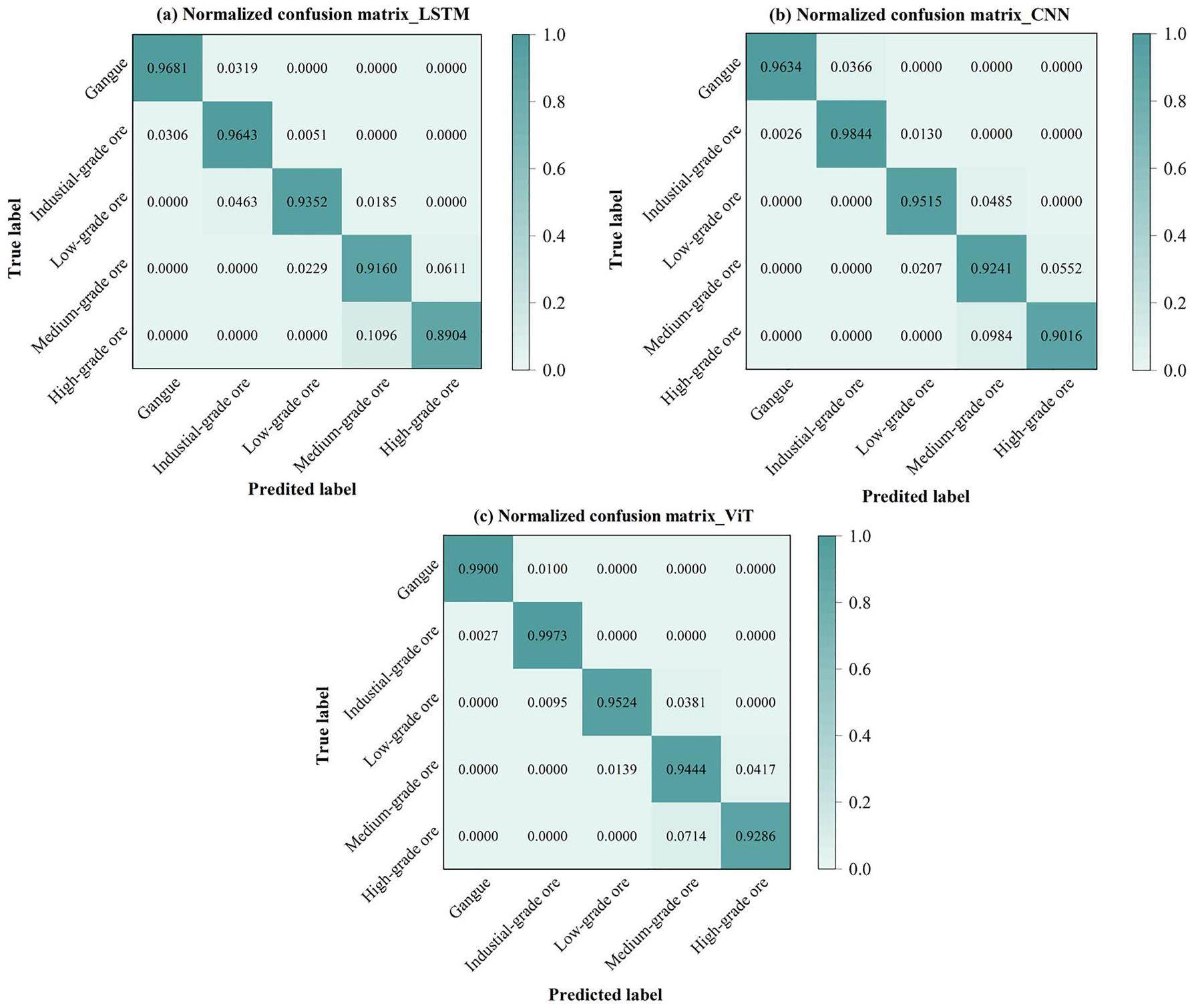
Figure 8 shows the confusion matrix for the copper ore grade identification. The diagonal elements of the confusion matrix denote the proportions of accurately classified copper ore grades. Combined with Table 4, it can be inferred that the highest accuracy rate was achieved for gangue and industrial-grade copper ores. All three models had accuracies of greater than 96%. Such high accuracy is attributed to the significant mineral differences between gangue and industrial-grade copper ores as well as their typical ore structures. High-grade copper ores exhibited the highest rate of misidentification and were often misclassified as medium-grade ores. There are two reasons for this finding. The first is that the difference between high- and medium-grade ores is small and easily confused, and the second is that high-grade copper ores often contain Fe. Because the characteristic peaks of Fe (7.631 MeV and 7.645 MeV) are similar to those of copper (7.64 MeV and 7.91 MeV), Fe affects the identification of high-grade copper ores. In identifying medium- and high-grade copper ores, the ViT model outperformed the LSTM and CNN models with a prediction accuracy of more than 92%.
Identification of associated minerals
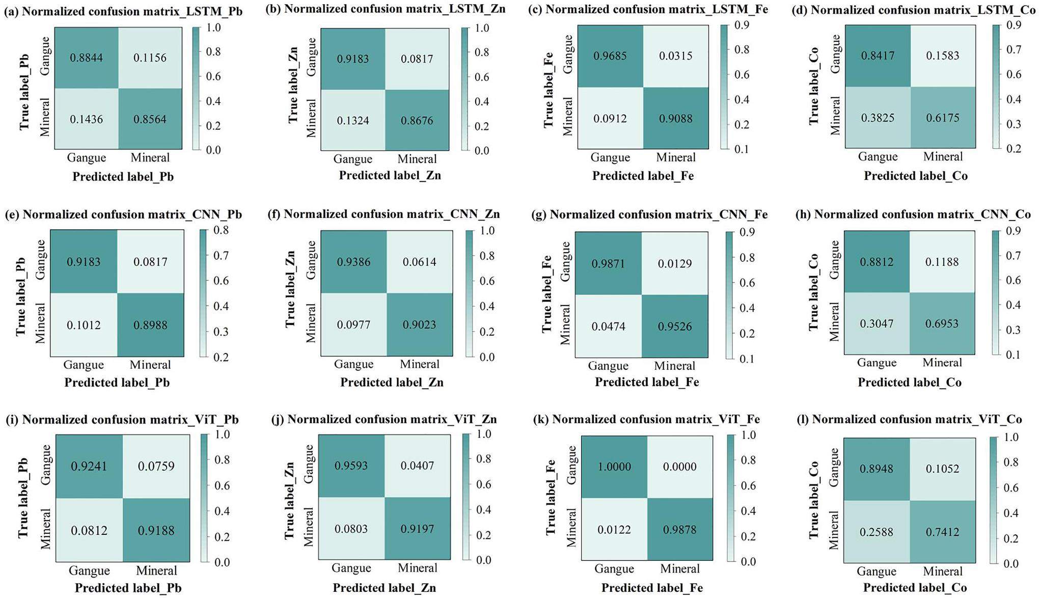
In the identification of associated minerals, the positive class was associated with minerals and the negative class was associated with gangue. Minerals associated with copper mines include Pb, Zn, Fe, and Co. Table 5 shows the identification results of the LSTM, CNN, and proposed ViT models for the minerals associated with copper ore. As shown in Table 5, the identification of the ViT model of associated minerals was significantly better than those of the other two models, and the performance ranking was ViT > CNN > LSTM. ViT had the best evaluation indicators, with average accuracy, precision, recall, F1 score, and F1(-) score values of 0.9222, 0.9278, 0.8919, 0.9091, and 0.9308, respectively. This analysis shows that ViT is the most effective method for classifying and identifying associated minerals and gangue.
| Model | Class | Accuracy | Precision | Recall | F1 score | F1(-) score |
|---|---|---|---|---|---|---|
| LSTM | Pb | 0.8711 | 0.8713 | 0.8564 | 0.8638 | 0.8776 |
| Zn | 0.8938 | 0.9084 | 0.8676 | 0.8875 | 0.8995 | |
| Fe | 0.9482 | 0.9373 | 0.9088 | 0.9228 | 0.961 | |
| Co | 0.7434 | 0.7528 | 0.6175 | 0.6785 | 0.7866 | |
| Macro average | 0.8641 | 0.8675 | 0.8126 | 0.8382 | 0.8812 | |
| CNN | Pb | 0.9091 | 0.9075 | 0.8988 | 0.9031 | 0.9143 |
| Zn | 0.9205 | 0.9363 | 0.9023 | 0.919 | 0.9219 | |
| Fe | 0.9771 | 0.9679 | 0.9526 | 0.9602 | 0.9839 | |
| Co | 0.8019 | 0.8132 | 0.6953 | 0.7497 | 0.8361 | |
| Macro average | 0.9022 | 0.9062 | 0.8623 | 0.8830 | 0.9141 | |
| ViT | Pb | 0.9215 | 0.9209 | 0.9188 | 0.9199 | 0.9231 |
| Zn | 0.9396 | 0.957 | 0.9197 | 0.938 | 0.9412 | |
| Fe | 0.9966 | 1.0000 | 0.9878 | 0.9938 | 0.9976 | |
| Co | 0.8311 | 0.8333 | 0.7412 | 0.7846 | 0.8611 | |
| Macro average | 0.9222 | 0.9278 | 0.8919 | 0.9091 | 0.9308 |
Figure 9 shows the confusion matrix of the associated mineral identification using the LSTM, CNN, and ViT models. This figure shows that Fe is most accurately identified among all elements. A possible reason for this is that the capture cross-section of Fe is large and the boundary grade is high. Co has the highest rate of misclassification. The LSTM, CNN, and ViT models often failed to identify the presence of Co in minerals. This is because the cutoff grade of Co was low (0.01%). Therefore, the low intensity of the characteristic gamma rays induced by the reaction between Co and neutrons makes it difficult to determine the presence of Co in the ore. The ViT model outperformed the other classification methods in identifying Co. In general, the ViT method achieved the best classification performance, particularly for Fe. The main reason for this is that, compared with other competing classifiers, the ViT model employs a self-attention mechanism to establish a global association of energy spectrum data, thus allowing the model to capture information from the entire gamma energy spectrum and improve the accuracy of identification.
Conclusion
A high-precision grade-identification method combining machine learning and PGNAA was proposed. First, a PGNAA measurement model was established using the Monte Carlo method. Subsequently, the structural parameters of the measurement device were optimized using MCNP. The resulting ViT model was trained and tested using a gamma energy spectrum dataset to identify the grade of copper ore and its associated minerals. These results demonstrated that the ViT model can effectively distinguish between different grades of copper ore. The average accuracy, precision, recall, F1 score, and F1(-) score values of identifying copper grades were 0.9795, 0.9637, 0.9614, 0.9625, and 0.9942, respectively. Furthermore, the model effectively recognized the associated minerals Pb, Zn, Fe, and Co. The identification accuracies of these associated minerals were 0.9215, 0.9396, 0.9966, and 0.8311, respectively.
Although the ViT model could effectively achieve the grade identification of copper ores and associated minerals, the action mechanism of the ViT model remains unclear. Therefore, the interpretability of grade identification achieved by the ViT model should be a focus of future research. The training and testing sets for the ViT model were obtained using Monte Carlo simulations. In future studies, we will consider using measured data to further validate the identification provided by the ViT model.
Errors and uncertainty in mineral resource and ore reserve estimation: The importance of getting it right
. Explor. Min. Geol. 11, 77-98 (2002). https://doi.org/10.2113/11.1-4.77Mineral resources evaluation with mining selectivity and information effect
. Funct. Fillers Nanoscale Miner. 37, 965-979 (2020). https://doi.org/10.1007/s42461-020-00229-2Practical way to quantify minerals from chemical assays at Malmberget iron ore operations–An important tool for the geometallurgical program
. Miner. Eng. 49, 7-16 (2013). https://doi.org/10.1016/j.mineng.2013.04.005Chemical analysis of high-pressure metamorphic rocks by PGNAA: Comparison with results from XRF and solution ICP-MS
, J. Radioanal. Nucl. Chem. 265, 339-348 (2005). https://doi.org/10.1007/s10967-005-0830-6Application and quality control of core data for the development and validation of elemental spectroscopy log interpretation
. Petrophysics. 55, 392-414 (2014).https://doi.org/10.1007/978-3-319-71216-1Flux measurements for a DD neutron generator using neutron activation analysis
. Nucl. Sci. Tech. 29, 52 (2018). https://doi.org/10.1007/s41365-018-0385-1Detection of heavy metals in aqueous solution using PGNAA technique
. Nucl. Sci. Tech. 27, 12 (2016). https://doi.org/10.1007/s41365-016-0010-0In situ determination of sulphur in coal seams and overburden rock by PGNAA
. Nucl. Instrum. Methods Phys. Res., Sect. B. 213, 530-534 (2004). https://doi.org/10.1016/S0168-583X(03)01623-9Response of a PGNAA setup for pozzolan-based cement concrete specimens
. Appl. Radiat. Isot. 68, 635-638 (2010). https://doi.org/10.1016/j.apradiso.2009.09.016Feasibility study of fast neutron-induced gamma ray imaging of large sample based on DT neutron generato
. Nucl. Instrum. Methods Phys. Res., Sect. B. 492, 7-14 (2021). https://doi.org/10.1016/j.nimb.2021.01.014Element analysis method of concealed explosive based on TNA
. Nucl. Sci. Tech. 30, 6 (2019). https://doi.org/10.1007/s41365-018-0527-5Advanced algorithms for retrieving pileup peaks of digital alpha spectroscopy using antlions and particle swarm optimizations
. Nucl. Sci. Tech. 31, 37 (2020). https://doi.org/10.1007/s41365-020-0745-5An inversion decomposition method for better energy resolution of NaI (Tl) scintillation detectors based on a Gaussian response matrix
. Nucl. Sci. Tech. 27, 58 (2016). https://doi.org/10.1007/s41365-016-0062-1Unfolding analysis of LaBr3: Ce gamma spectrum with a detector response matrix constructing algorithm based on energy resolution calibration
. Nucl. Sci. Tech. 29, 1 (2018). https://doi.org/10.1007/s41365-017-0340-6Source-less density measurement using an adaptive neutron-induced gamma correction method
. Nucl. Sci. Tech. 34, 125 (2023). https://doi.org/10.1007/s41365-023-01274-4A method for neutron-induced gamma spectra decomposition analysis based on Geant4 simulation
. Nucl. Sci. Tech. 33, 154 (2022). https://doi.org/10.1007/s41365-022-01144-5Optimization study on neutron spectrum unfolding based on the least-squares method
. Nucl. Sci. Tech. 29, 118 (2018). https://doi.org/10.1007/s41365-018-0454-5Application of the Monte Carlo Library Least-Squares (MCLLS) approach for chromium quantitative analysis in aqueous solution
. Appl. Radiat. Isot. 150, 39-42 (2019). https://doi.org/10.1016/j.apradiso.2019.02.018Experimental optimization of a landmine detection facility using PGNAA method
. Nucl. Sci. Tech. 19, 109-112 (2008). https://doi.org/10.1016/S1001-042(08)60033-0A bulk analysis system using the prompt gamma neutron activation method and neural network
. Eur. Phys. J. Plus. 132, 273 (2017). https://doi.org/10.1140/epjp/i2017-11533-6A quantitative PGNAA study for use in aqueous solution measurements using Am–Be neutron source and BGO scintillation detector
. Nucl. Instrum. Methods Phys. Res., Sect. A. 808, 123-127 (2016). https://doi.org/10.1016/j.nima.2015.11.070Research on PGNAA adaptive analysis method with BP neural network
. Mod. Phys. Lett. B. 30, 32-33 (2016). https://doi.org/10.1142/S0217984916503863Processing scintillation gamma-ray spectra by artificial neural network
. J. Radioanal. Nucl. Chem. 325, 471-483 (2020). https://doi.org/10.1007/s10967-020-07239-wTowards sustainable copper matrix composites: manufacturing routes with structural
. J. Compos. Mater. 54, 19 (2020). https://doi.org/10.1177/0021998319900655The application of PGNAA borehole logging for copper grade estimation at Chuquicamata mine
. Appl. Radiat. Isot. 60, 771-777 (2004). https://doi.org/10.1016/j.apradiso.2003.12.007Monte Carlo simulation of Cu, Ni and Fe grade determination in borehole by PGNAA technique
. J. Radioanal. Nucl. Chem. 315, 51-56 (2018). https://doi.org/10.1007/s10967-017-5636-9Prompt gamma neutron activation analysis method and instrumentation for copper grade estimation in large diameter blast holes
. Appl. Radiat. Isot. 59, 197-203 (2003). https://doi.org/10.1016/S0969-8043(03)00163-5Study on element detection and its correction in iron ore concentrate based on a prompt gamma-neutron activation analysis system
. Nucl. Sci. Tech. 30, 58 (2019). https://doi.org/10.1007/s41365-019-0579-1Identification of Pb–Zn ore under the condition of low count rate detection of slim hole based on PGNAA technology
. Nucl. Eng. Technol. 55, 1708-1717 (2023). https://doi.org/10.1016/j.net.2023.01.005Gradient boosting decision tree for lithology identification with well logs: A case study of zhaoxian gold deposit
. Nat. Resour. Res. 30, 3197-3217 (2021). https://doi.org/10.1007/s11053-021-09894-6Produced water characterization by prompt gamma-ray neutron activation analysis
. Meas. Sci. Technol. 22,The optimization of coal on-line analysis system based on signal-to-noise ratio evaluation
. J. Radioanal. Nucl. Chem. 318, 1279-1286 (2018). https://doi.org/10.1007/s10967-018-6173-xOptimization of moderator assembly for neutron flux measurement: experimental and theoretical approaches
. Nucl. Sci. Tech. 228, 61 (2017). https://doi.org/10.1007/s41365-017-0213-zDesign of the explosion-proof detection integrated system based on PGNAA technology
. J. Radioanal. Nucl. Chem. 322, 1719-1728 (2019). https://doi.org/10.1007/s10967-019-06837-7Attention is all you need
. arXiv:1706.03762. https://doi.org/10.48550/arXiv.1706.03762An image is worth 16x16 words: Transformers for image recognition at scale
. arXiv:2010.11929. https://doi.org/10.48550/arXiv.2010.11929Classification assessment methods
. Appl. Comput. Inf. 17, 168-192 (2020). https://doi.org/10.1016/j.aci.2018.08.003The effect of microwave radiation upon the processing of Neves Corvo copper ore
. Int. J. Miner. Process. 63, 29-44 (2001). https://doi.org/10.1016/S0301-7516(00)00069-7Platinum-copper-nickel and platinum ores of Norilsk region and their ore mineralization
. Russ. J. Gen. Chem. 81, 1288-1301 (2011). https://doi.org/10.1134/S1070363211060351Reliable Accuracy Estimates from k-Fold Cross Validation
. IEEE Trans. Knowl. and Data Eng. 32, 1586-1594 (2020). https://doi.org/10.1109/TKDE.2019.2912815The authors declare that they have no competing interests.

