Introduction
The China Initiative Accelerator Driven System (CiADS) [1], currently under construction, employs a high-power linear accelerator at its front-end to generate a 500 MeV proton beam with an intensity of 5 mA [2-4]. To verify the feasibility of a continuous wave (CW) proton beam with a current of 10 mA, the China ADS Front-End Demo Linac (CAFe) was built. In March 2021, CAFe achieved its design goal with the successful commissioning of a 10 mA, 205 kW CW proton beam at an energy of 20 MeV [5].
The synthesis and property study of superheavy nuclei is an important frontier and one of the difficulties in current nuclear physics [6-10]. Since 2021, the CAFe facility had been upgraded to CAFE2 (China Accelerator Facility for superheavy Elements) for the exploration of new isotopes with an operating beam intensity of approximately 10 pμA [11, 12]. The layout of CAFE2, as shown in Fig. 1, includes both normal conducting and superconducting (SC) sections, and a new gas-filled recoil separator, SHANS2 (Spectrometer for Heavy Atoms and Nuclear Structure-2), was constructed at the end of the beam line [13].
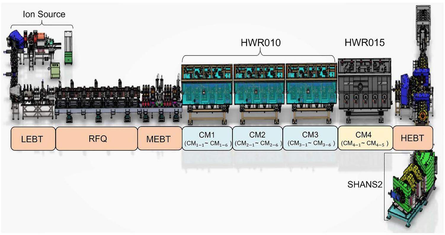
The SC section contains a total of 23 SC half-wave resonator (HWR) cavities assembled in four cryomodules (CM1–CM4) and regulated with an individual digital low-level radio-frequency (LLRF) system, in which CM1 to CM3 are each equipped with six HWR010 cavities, while CM4 is equipped with five HWR015 cavities [5, 14-16]. HWR010 and HWR015 are two cavity types named according to their optimal β value, with their operational parameters are shown in Table 1.
| Cavity | HWR010 (CM1~CM3) | HWR015 (CM4) |
|---|---|---|
| QL (arb.units) | 3×10⁵~10×105 | 6×10⁵~8×10⁵ |
| f0.5 (Hz) | 81.25~270.0 | 101.5~135.4 |
| fRF (MHz) | 162.5 | 162.5 |
| Norm. shunt impedance (Ω) | 225 | 382 |
| Vc/Epeak (m) | 0.038 | 0.066 |
| Epeak (MV/m) | 25~35 | ~30 |
| Opt. β (v/c) (arb.units) | 0.10 | 0.15 |
| KLFD (Hz/(MV/m)2) | -0.4~-0.2 | ~-0.2 |
To meet the high demand for beam availability in the future CiADS, the research team at the Institute of Modern Physics is working diligently to enhance the reliability of various subsystems of the CAFE2. However, owing to the stringent operating conditions of the SC cavities (high power, electric field, and frequency) and the extremely narrow operating bandwidth [17], cavity failures easily occur when subjected to disturbances (e.g., mechanical vibrations). The operational experiences from different accelerator laboratories have revealed that the leading causes of short machine downtime trips are SRF faults [18-20]. Rapidly identifying the causes of faults and reducing the SC cavity failure rate for stable operation of the accelerator are imperative.
When an RF fault occurs, the LLRF's data acquisition (DAQ) system simultaneously records 16 RF signals from each cavity, providing comprehensive fault information. This process is triggered when the LLRF system for any cavity in a cryomodule detects a fault condition (e.g., field fluctuation beyond the tolerance limit). Based on this data, system experts can analyze the fault types and causes to comprehend the underlying physical mechanisms. To implement appropriate measures for fault handling, the accurate and swift identification of fault patterns is essential. However, the diversity of fault modes and the similarity of fault characteristics complicate fault analysis. Although control-room operators have access to raw waveform data captured during fault occurrences, correctly interpreting the signals requires expertise. Additionally, a fault in one pattern can trigger a different pattern through several physics effects, and a fault in a single SC cavity may propagate to the adjacent cavities, leading to group faults in a cryomodule. In such cases, providing near real-time fault feedback is rather crucial for control-room operators.
Identifying the offending cavity with existing software and hardware is difficult to do automatically. Traditional methods are generally limited by the requirement of expertise and cannot quickly process large amounts of fault data. In recent years, machine learning (ML) methods have made remarkable progress in pattern recognition tasks and are widely used in various fields [21]. As a data-driven algorithm, ML shows potential applications in particle accelerators, such as beam optimization, intelligent control system, anomaly detection, and fault diagnosis [22-27]. For fault-pattern recognition of SC cavities, the challenge lies in solving a multidimensional time-series classification problem. SC cavity faults occur in milliseconds or microseconds; therefore, a high sampling rate is required to capture the signal features when the fault occurs. However, existing time-series feature-extraction models, such as long short-term memory (LSTM) and gated recurrent units (GRU), cannot process such a long sequence, and the fault information is lost in the data after downsampling [28]. Therefore, implementing feature engineering is vital for fault identification. At the Jefferson Laboratory (JLab), the Continuous Electron Beam Accelerator Facility (CEBAF) uses the autoregression (AR) method to extract features from the cavity voltage and the incident and reflected voltages, and builds an ML-based fault classification model [18]. Compared to expert results, the method achieves a classification accuracy of 82%. Research results from CEBAF indicate that the performance of the ML method in identifying abrupt faults (e.g., LLRF control trips and E-quench faults) is unsatisfactory [18, 29]. This may be primarily attributed to the limitations of AR methods in extracting non-stationary signals.
In this work, we introduce an expert knowledge–driven approach to feature engineering construction, aiming to address the limitations of existing methods in automated fault identification. We analyzed the historical data generated via the operation of the CAFE2 and categorized the SC cavity faults into eight types. Based on the formation mechanism and waveform characteristics of different faults, we designed reasonable feature engineering to transform raw data into an intermediate representation that expresses the underlying data patterns. Subsequently, we evaluated the effect of feature engineering on CAFE2 through two aspects: confusion matrix and information gain, to obtain a comprehensive understanding of its impact on model performance. Finally, fault analysis was conducted on the historical data of CAFE2 operation, tallying the most prevalent fault types for each cavity. This analysis provides valuable guidance for the future maintenance and upgrade of SC cavities, enabling the development of preventive measures against common faults as well as the optimization of maintenance strategies to ensure system stability and sustained high-efficiency operation.
The remainder of this paper is organized as follows. In Sect. 2, the method for acquiring offline fault data of the SC cavity is introduced and the criteria for labeling fault types are discussed. In Sect. 3, the development of ML models is discussed, including the calibration of the raw data, the implementation of feature engineering, and the theory of ensemble learning methods. Finally, the performance evaluation of the aforementioned method based on 2023 operational data is presented, followed by a discussion regarding future research.
Data analysis and labeling
Data acquisition
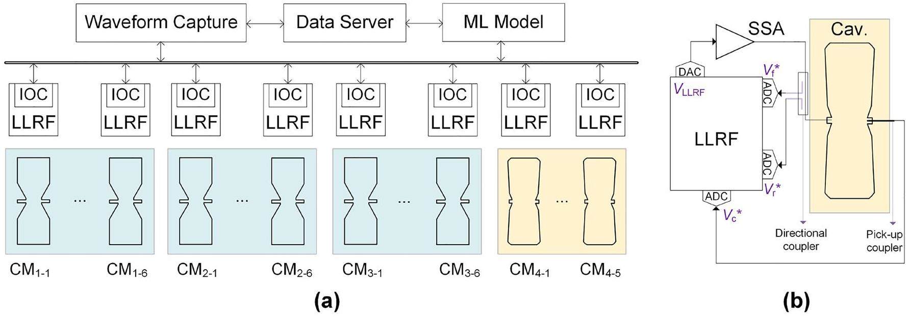
For each cavity fault, the newly developed DAQ system synchronously captures timestamps and saves waveform records of 16 RF signals from each of the cavities in the cryomodule. The DAQ system comprises LLRF and EPICS (experimental physics and industrial control systems) components along with various high-level applications that collaborate to collect and store data for subsequent offline analyses and inspections.
A waveform capture module was developed to gather RF time-series signals after a fault occurrence and write them to a file for later analysis. Each of the 16 harvested waveform signals comprises 50000 points. The trigger is configured such that approximately 80% of the recorded data precede the fault, whereas 20% follow the fault. Subsequently, the collected waveform data are written to network storage and uploaded to a data server via a waveform-specific web service. Finally, all waveform-related data are backed up online indefinitely to tape daily and compressed monthly to reduce online storage (Fig. 2.
According to the different research requirements of CAFE2, the sampling rate is typically adjusted within the range of 10 kHz to 100 kHz (based on the dominant fault pattern of the specific cavity), resulting in approximately 0.5-5 s of fault data. As the feature-engineering method proposed in this study is not affected by the sampling rate, we extract 0.5 s segments from all fault waveforms as the raw data for feature engineering, of which 80% is pre-fault information and 20% is post-fault information.
Data labeling
We analyzed the fault data generated by the 23 SC cavities of the CAFE2 accelerator between January 2023 and November 2023 and labeled 1932 typical samples for supervised learning. When a fault is triggered in the SC cavity, the low-level system sends 16 channels of the RF signals to the data server. Notably, these 16 channel signals include 6 real measurement signals extracted using a pick-up coupler and directional coupler, as well as 10 control signals generated internally within the FPGA (e.g., feedforward signals for pulse beam compensation or calibration signals). In this work, the cavity voltage (
| Name | Definition |
|---|---|
| Vc | Maximum accelerating voltage acting on the beam. |
| Vf | Forward wave sent from the RF generator (e.g., SSA). |
| Vr | Backward wave reflected from the cavity input coupler back to the RF generator. |
| f0.5 | Frequency bandwidth where the voltage drops to |
| Δf | Frequency difference between the RF generator frequency (fRF) and the cavity resonance frequency (f0), expressed as |
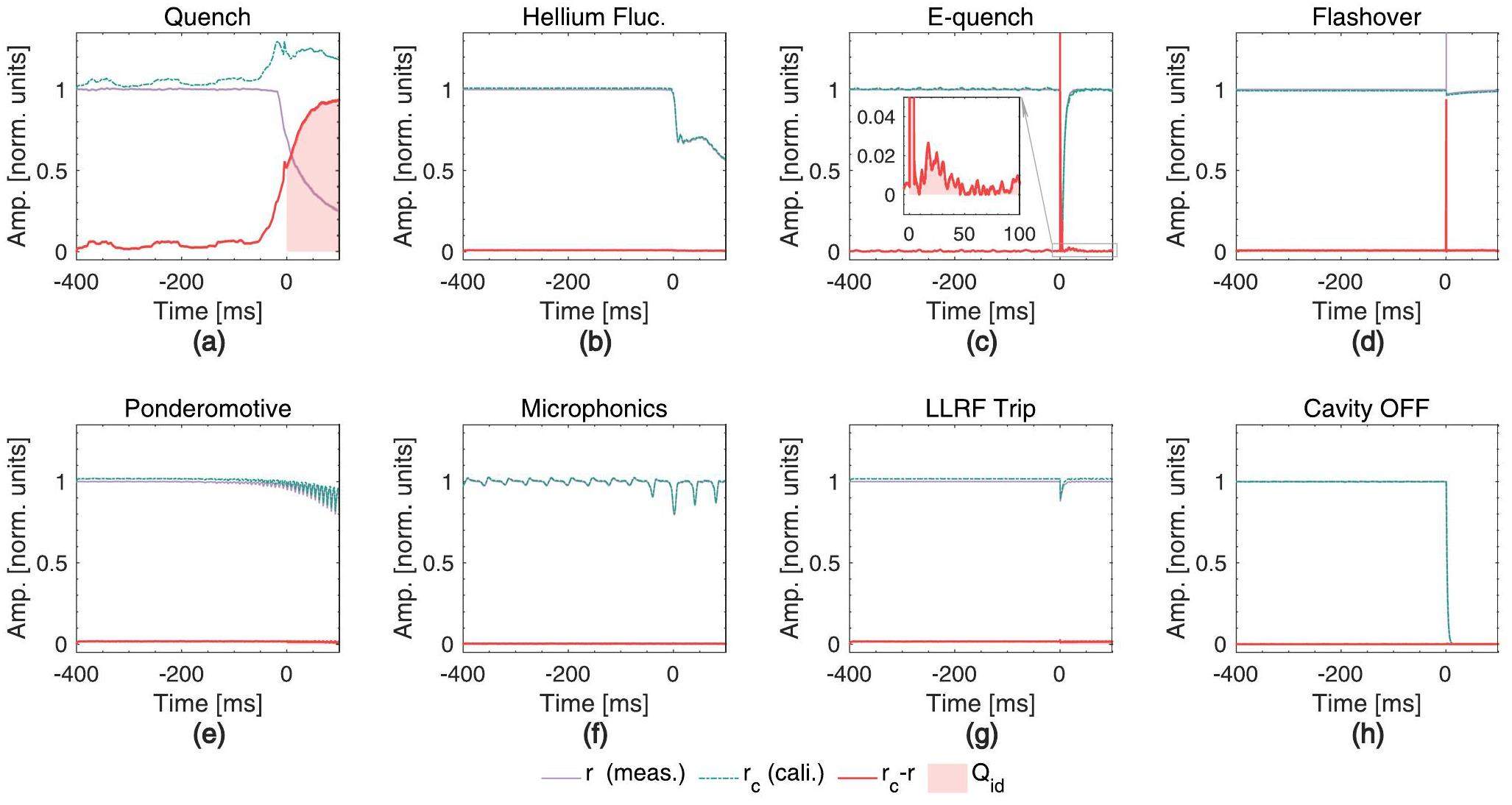
Based on these signals, we summarize eight fault modes: thermal quench (quench), helium pressure fluctuations (helium fluc), electrical quench (E-quench), flashover, microphonics, ponderomotive, LLRF trip, and single-cavity off (cavity off), as shown in Fig. 3. Notably, during the commissioning phase of CAFe, faults induced by transient beam- loading effects with a beam current of 10 mA are common; however, with CAFE2 operating in the CW mode at microampere-level beam currents, this fault pattern is essentially absent [30, 31]. We briefly describe the process of fault-signal analysis and labeling from the perspective of system experts.
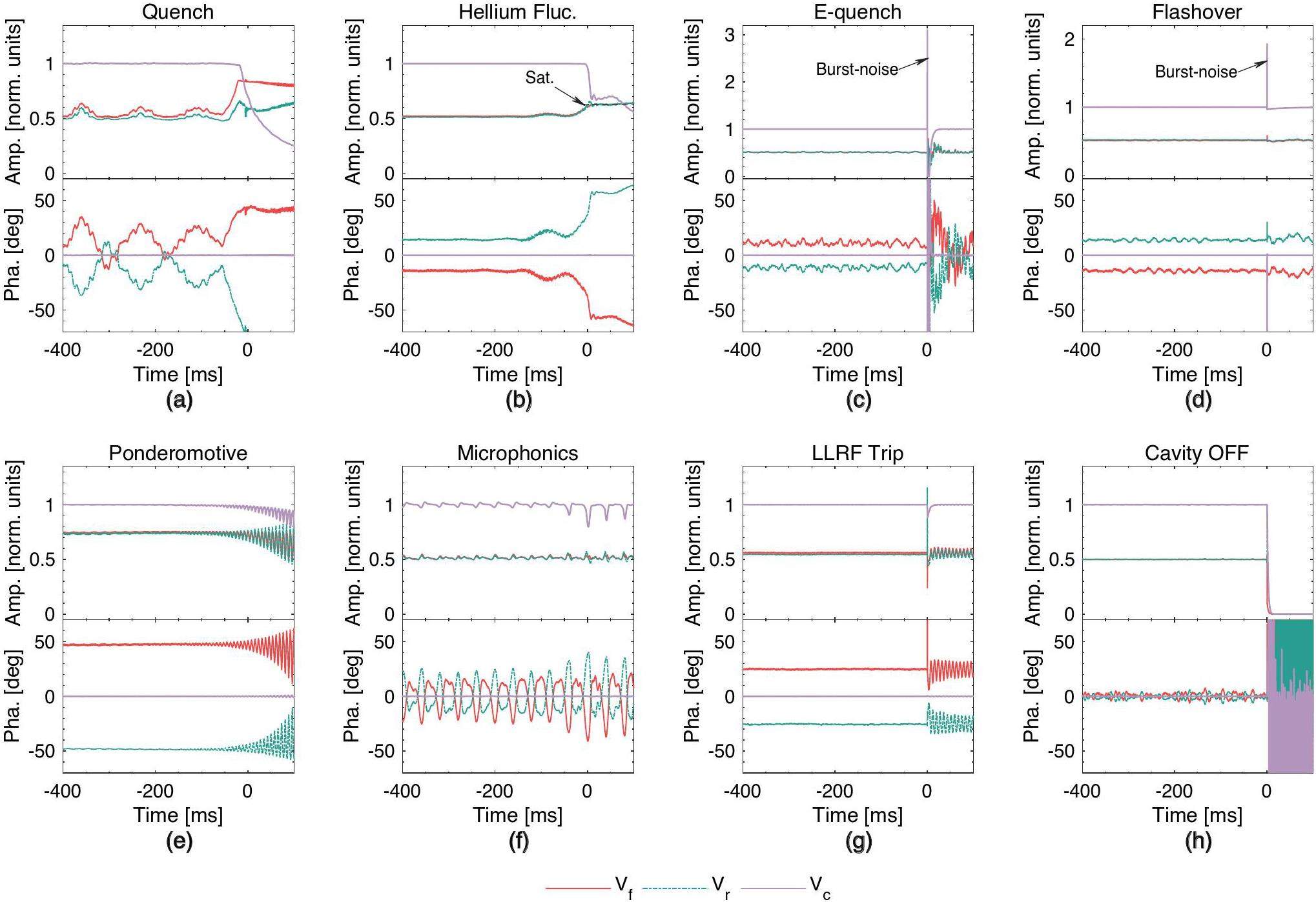
Quenching refers to the localized overheating of the SC cavity wall, which results in the premature breakdown of superconductivity (thermal breakdown). A quench typically manifests as a rapid drop in the unloaded quality factor (Q0) and the loaded quality factor (QL). When a fault occurs, the cavity's QL and detuning can be solved according to Vc and Vf, respectively, as shown in Eq. (1) [32].
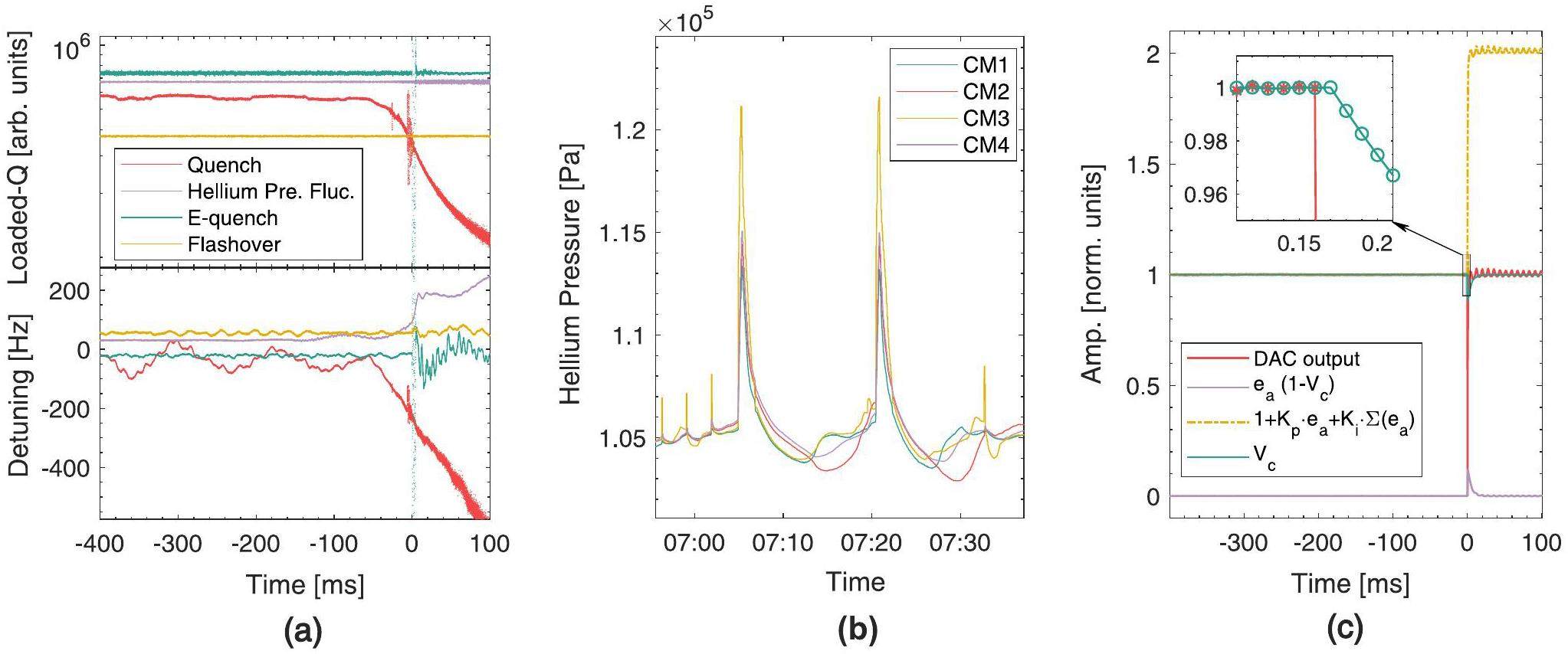
Quenches induce changes in the heat load of the cryosystem, resulting in rapid fluctuations in helium pressure over a short period, ultimately causing the SC cavities within the cryomodule to undergo considerable detuning on the millisecond scale. When detuning exceeds the cavity bandwidth, the power source output reaches saturation and eventually triggers multiple cavity faults (Fig. 5a. Typically, helium pressure fluctuations (helium flucs) are secondary faults that are induced by quenching. However, in a few cases (e.g., SC magnet quenching or cryogenic system control logic faults), we observed simultaneous helium pressure changes in the four cryosystems without any cavities experiencing quenching (Fig. 4b. In this study, we labeled these fault patterns as helium flucs.
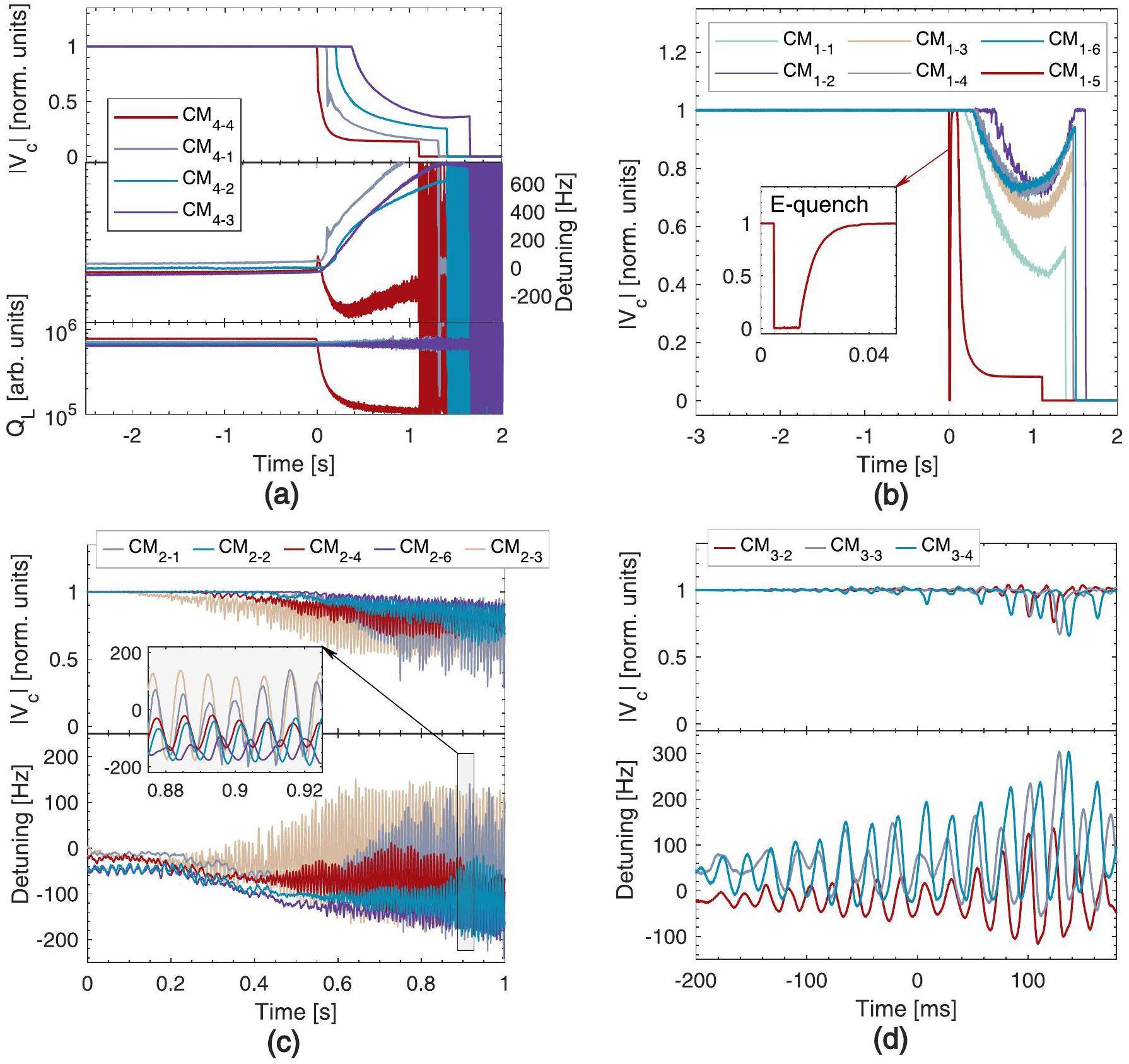
E-quench typically manifests as a sudden and complete loss of stored energy in the cavity. JLAB interpreted this loss as the effect of the release of numerous electrons inside the cavity, which absorbed the cavity energy. A flashover involves an FE-initiated discharge on an RF ceramic window surface [33, 18]. It typically does not cause any Vc degradation but can result in burst noise in the cavity's pick-up signal. Notably, E-quench can also be accompanied by burst noise events. The main difference between the two is that E-quench can cause total or partial gradient loss, whereas flashover does not cause such a loss [34]. Experience from CAFE2 operations suggests that when the gradient loss exceeds 30%, E-quench may further trigger a quench fault and cause multiple cavity failures within the same cryomodule (Fig. 5b. Conversely, when the gradient loss is less than 30%, multiple cavity failures generally do not occur. Therefore, in this work, we categorize E-quench events with gradient loss less than 30% as “flashover” faults, and those with gradient loss greater than 30% as “E-quench” faults.
Ponderomotive oscillatory instabilities result from the nonlinear coupling between the electrical and mechanical modes of the cavity, which is accompanied by an accelerating gradient and detuning that begins to oscillate with increasing amplitude [35]. Based on measurements of the cavity mechanical mode transfer function, most cavities exhibit a significant mechanical mode around 125 Hz [36]. As shown in Fig. 5c, when a cavity undergoes oscillations due to the ponderomotive effect, the oscillations in the cavity can be transmitted to other cavities, resulting in a multicavity fault. Notably, the formation of ponderomotive oscillations depends on factors such as feedback parameters, Lorentz detuning coefficient, and cavity detuning [37, 38]. In this example, no ponderomotive oscillations are observed in CM2-5.
Microphonics are changes in the cavity frequency caused by connections to the external world, such as vacuum pump vibrations, at a frequency generally less than 50 Hz. Compared with ponderomotive instability, cavity detuning induced by microphonics is determined by external vibration sources, with the oscillation energy typically not exhibiting divergent growth. As shown in Fig. 5d, microphonics typically occur in multiple cavities. Notably, microphonics and helium flucs are commonly grouped as microphonic faults [35]. In this study, we specifically distinguished between vibration-dominated and non-vibration-dominated (e.g., cryogenic system-dominated) cases. Therefore, we categorized these into two fault modes.
There are many possible causes of LLRF faults, such as electronics being affected by radiation showers in the tunnel, leading to single-event upsets that flip a bit in the digital data stream [39]. In CAFE2, the most common type of LLRF fault is triggered by the control logic inside the FPGA. As shown in Fig. 4c, around 0 ms, the DAC output suddenly drops to zero, causing a transient fluctuation in Vc and triggering a fault. We carefully checked the internal logic of the LLRF but found no issues. One possible reason is that clock glitches disturb the accumulator of the proportional-integral (PI) controller. The yellow curve in Fig. 4c shows the PI output obtained from the simulation based on the input of the PI controller, which differs from the DAC output by a fixed constant. LLRF faults are generally single-issue faults, implying that they do not cause further faults in multiple cavities. Similar to the case in the CEBAF [18], we classify “cavity turn off” events triggered by external machine interlock signals as “cavity off” modes, including arc interlock or RF source interlock.
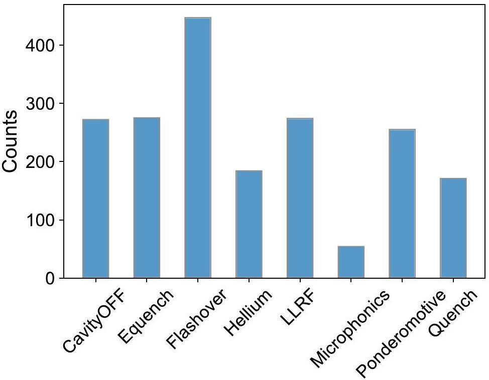
Based on the above steps, we completed data annotation and labeled a total of 1932 fault events. The distribution of sample counts for each fault type is shown in Fig. 6. Because the first cavity to trigger a fault can usually be determined based on the time of the fault occurrence, in this study, we focused on identifying the fault type of the source cavity.
Machine learning method
For fault pattern recognition in an SC cavity, the challenge lies in solving a multidimensional time-series classification problem. In this section, we introduce how to extract fault-related features from raw RF signals and construct a machine-learning model.
Data preprocessing
The cavity voltage (
Subsequently, the three signals were normalized relative to
Feature engineering
The success of ML methods often depends on data and features, with feature engineering playing a crucial role and directly affecting the performance, generalization, and interpretability of the models. Fig. 3 shows the amplitude and phase changes in Vc, Vf, and Vr recorded by the LLRF system when a fault occurs in the SC cavity. Based on the experience of experts in inferring fault types, we extracted eight features related to fault types, which were calculated from the amplitudes and phases of Vc, Vf, and Vr. These features serve as intermediate representations of the raw data and are employed as model inputs. The following section introduces the calculation methods for the eight features.
First, we introduce the thermal quenching (quenching) recognition feature Qid. When a cavity quenches, its QL decreases rapidly [43]. Although QL serves as a hallmark for distinguishing quench faults from other modes, its computational process requires solving the Vc differential equation (Eq. (1)), which is highly time consuming, whereas fault identification must be accomplished within milliseconds. Next, we introduce the quench identification features based on the cavity coefficient difference equation. Let
Let
Both ponderomotive and microphonics are related to mechanical vibrations, as shown in Fig. 3e and Fig. 3f, where Vc exhibits significant oscillatory characteristics. Given this, we apply fast Fourier transforms (FFT) to convert the detuning signal (
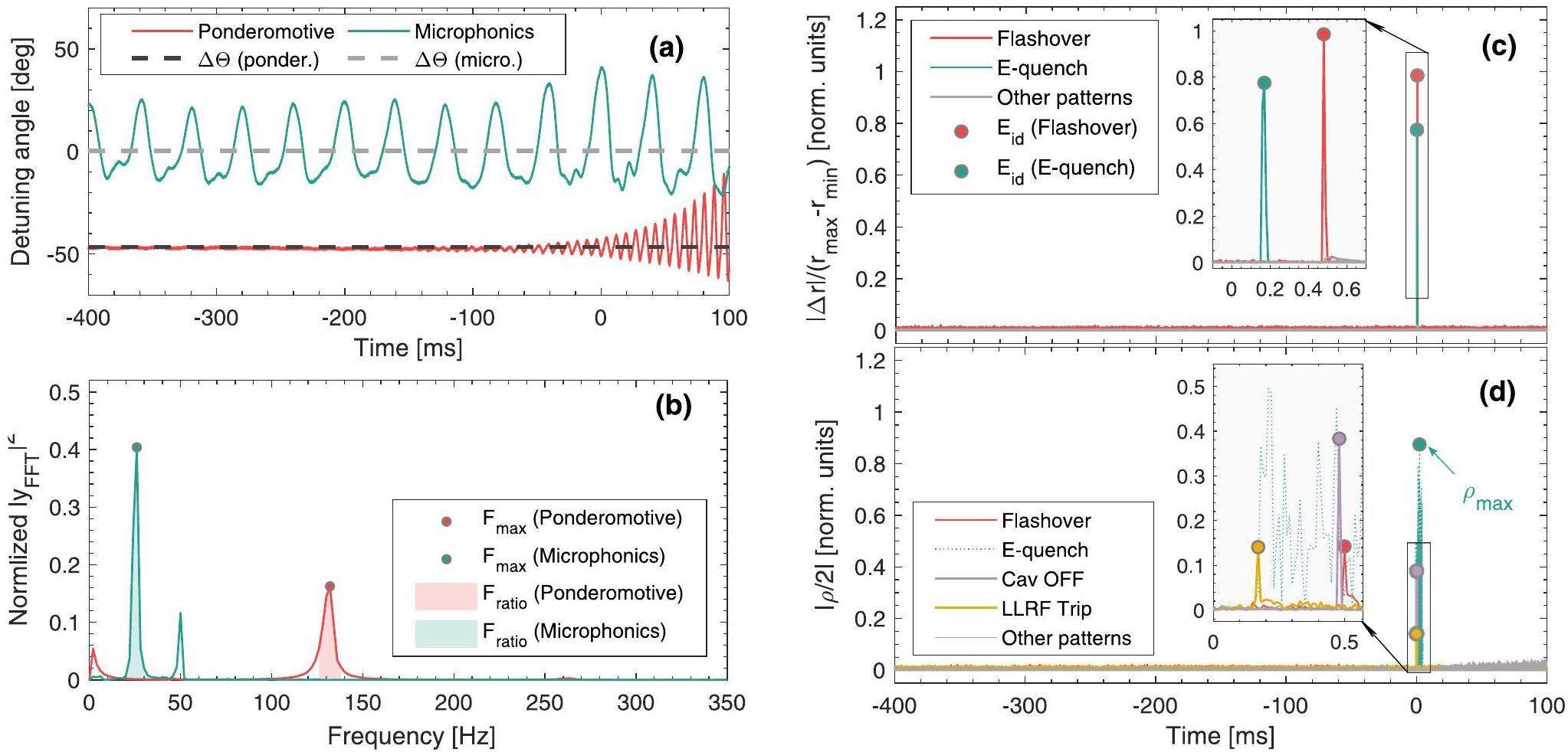
The flashover, E-quench, and LLRF trip faults induced a rapid change in the amplitude of Vc on the submillisecond timescale, exhibiting significant gradients at the transition points. We extracted the relative change in the amplitude of Vc as a learnable feature, denoted by Eid, to quantify the deviation of the transient signal from the baseline. The calculation is as follows:
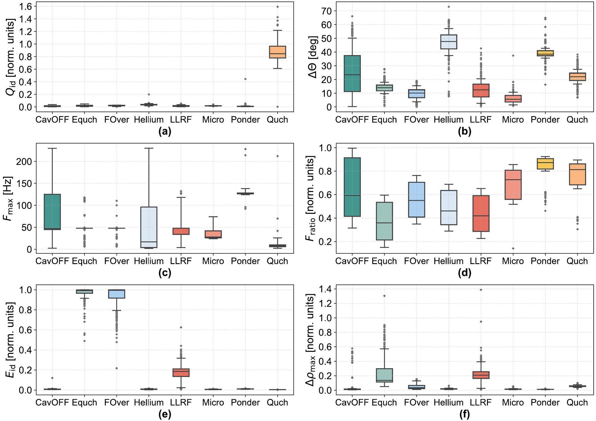
In the preceding section, we systematically clarified the theory and calculation methods of the designed expert features, from complex physical attributes to basic statistical features, which are of great significance to the analysis and decision-making processes as intermediate representations of the raw data. Table 3 lists simple definitions of the eight expert features. The distribution results for each feature in the 1932 labeled samples are shown in Fig. 9. As can be observed, except for the quench fault, it is challenging to distinguish other faults based on a single feature. Therefore, it is necessary to explore complex combinations of features.
| Feature | Definition |
|---|---|
| Qid | A quantity related to QL, mainly used to assess the physical properties of the cavity when a quench occurs. |
| The average cavity detuning angle for determining if a significant cavity detuning occurred after the fault. | |
| Fmax | The dominant frequency component in the cavity detuning angle spectrum (FFT result). |
| Fratio | The proportion of the energy of Fmax to the total energy, primarily used to determine if the cavity is undergoing vibration. |
| Eid | The relative change in the first-order difference of the Vc amplitude for detecting if the pick-up signal has undergone an abrupt change. |
| Δρmax | The maximum of the first-order difference of the Vf amplitude for checking whether the forward signal drops in a short time |
| rrms1 | rms radius of the amplitude in Vc before the fault occurs |
| rrms2 | rms radius of the amplitude in Vc after the fault occurs |
In addition to the aforementioned eight expert features, we employed the AR method to explore the autocorrelations within sequential data, capturing the trends and periodicities in the signal. In the AR method, it is assumed that the current value of a time series is correlated with several past values; that is, past observations impact the current value. This autocorrelation can be controlled by the order (p) of the AR model, where p indicates the extent to which past observations affect the current values. By linearly combining past observations to predict future values, a mathematical expression for AR can be obtained as follows [18]:
Ensemble learning models
Ensemble learning, an ML technique that combines the predictions of multiple models to improve overall performance, is widely used in various data-driven scenarios [45]. Ensemble models mitigate the weaknesses inherent in a single algorithm by aggregating diverse predictions, resulting in improved accuracy and robustness. Moreover, ensemble learning excels in handling complex and high-dimensional data, where individual models may struggle. The diversity introduced through different learning approaches or models helps reduce overfitting and provides a more generalized and reliable solution. Furthermore, ensemble methods, such as bagging and boosting, offer versatility across a spectrum of tasks, making them adaptable to different types of datasets and problems. Overall, exploiting the collective intelligence of multiple-model position ensemble learning is a powerful technique for optimizing the predictive outcomes of ML models.
Random Forest (RFs) is a model based on decision tree classifiers, using an ensemble approach that utilizes bagging among multiple decision trees [46]. The core idea behind bagging is to create multiple subsets of the original training dataset using random sampling with replacement. Each subset is used to train a separate base model. The final prediction is obtained by aggregating the predictions of all the individual base models, thereby reducing the risk of bias and variance associated with individual trees. For regression tasks, this aggregation is usually performed by averaging the predictions, whereas for classification tasks, a majority voting mechanism is often employed. The “random” in RFs stems from the introduction of randomness in two key aspects: bootstrap sampling and feature selection. Bootstrap sampling can generate multiple differentiated subsets to train a range of base models and is fundamental in ensemble learning methods such as bagging [47]. Feature selection refers to the process of selecting a subset of relevant features to construct individual decision trees within a forest. Instead of considering all available features to determine the best split at each node, only a randomly chosen subset of features is evaluated. This random selection of features introduces variability among trees because different trees may consider different features for splits, even if they are trained on the same data, which contributes to the robustness and generalization ability of the model. In RFs, the feature selection process is controlled by the key parameter “max_features”. Besides that, the “n_estimators” parameter specifies the number of trees in the forest; more trees generally improve accuracy but increase computational cost. The “max_depth” parameter controls the maximum depth of each tree; deeper trees capture more complex patterns but may overfit the data.
eXtreme Gradient Boosting (XGBoost) is a gradient boosting algorithm known for its efficiency and excellent predictive performance [48]. Unlike bagging methods that train models independently in parallel, boosting sequentially trains boosters (such as gbtree or gblinear), with each tree attempting to correct the errors of the previous tree with the aim of incrementally improving accuracy. The final prediction is the weighted sum of the predictions from all the individual trees. During the iterative training process, observations are assigned different weights based on their classification; misclassified observations are given more weight, whereas correctly classified observations are given less weight. This process is achieved by focusing on the model residuals, which directs the subsequent models to focus more on hard-to-predict cases. To prevent overfitting, XGBoost applies “shrinkage” during training, meaning it does not fully trust the residuals learned by each weak learner. This is achieved by multiplying the residual value that each weak learner fits by a “learning_rate” in the range of (0, 1]. A lower “learning_rate” makes the model more robust to overfitting by ensuring that each tree makes only a small adjustment to the model. This typically requires more trees to reach the same level of performance as a model with a higher “learning_rate”. Therefore, there is a trade-off between “learning_rate” and “n_estimators”. Additionally, XGBoost combines parameters such as “max_depth,” “gamma,” and regularization parameters (L1 and L2) to further reduce overfitting. It also uses “subsample” and “colsample_bytree” to introduce randomness by specifying the fraction of the training data and features used for each tree, respectively. A robust model can be achieved by coordinated optimization of these parameters.
Next, we separately evaluated the performances of the two ensemble learning methods in identifying SC cavity faults.
Results and discussion
Data visualization
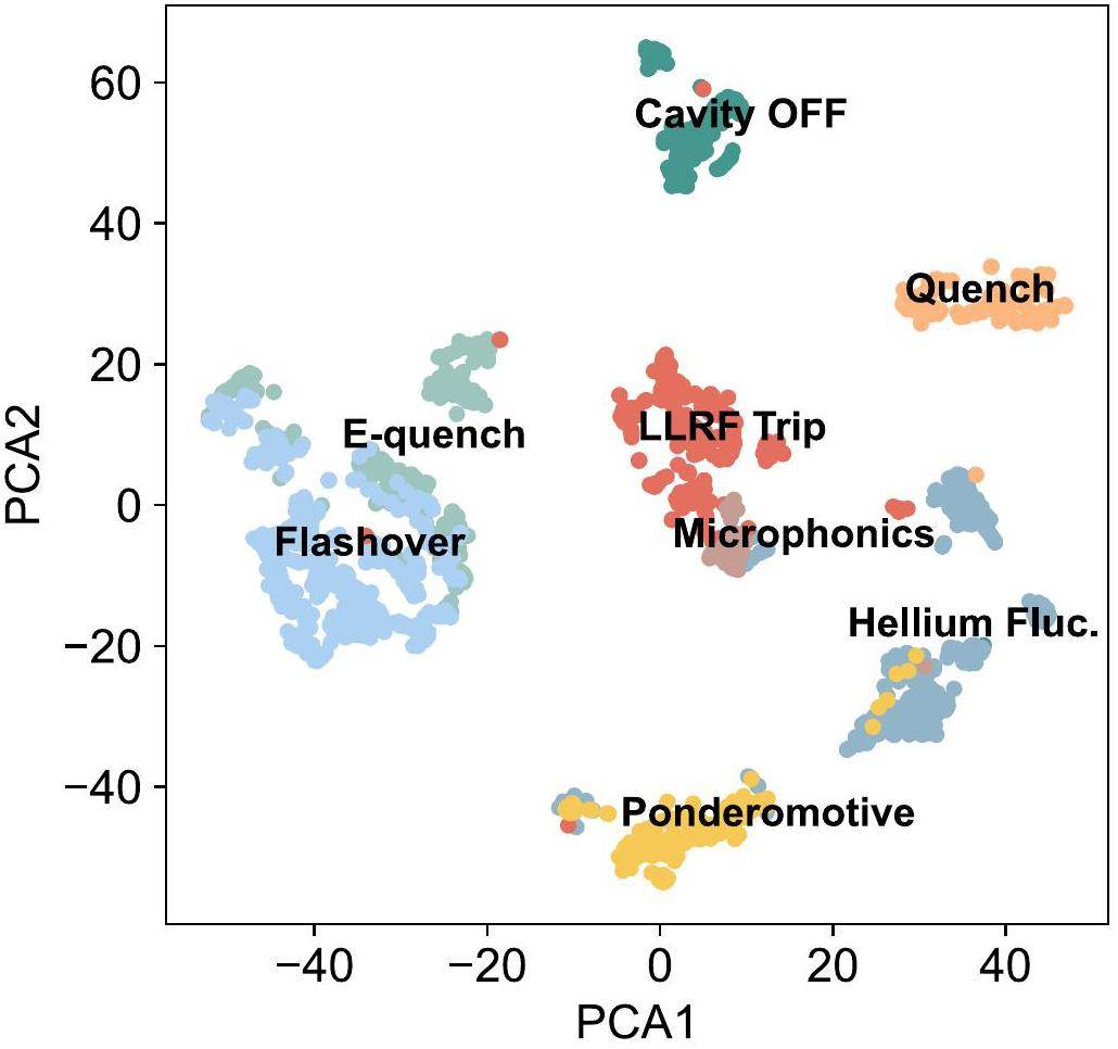
Before model training, we applied principal component analysis (PCA) to perform dimensionality reduction and visualized all samples in 2D coordinates. The results are shown in Fig. 10, where the clustering, distribution, and correlations within the data are clearly observed. This visualization aids experts in better understanding the data and uncovering potential relationships, thereby facilitating a more detailed categorization of the original dataset. Another important aspect of dimensionality-reduction visualization is the identification of outliers or anomalous points in each class to check for errors in the manual labeling process. Manual labeling requires a system expert to have considerable experience and intuition regarding SRF cavities operating with beams and to understand the complex physical mechanisms underlying the faults, for which PCA serves as a valuable auxiliary tool. Figure 10 indicates the presence of several outliers. After verification with domain experts, corrections were made to several erroneously labeled samples. For instance, a cavity-off fault was mislabeled as an LLRF trip, a helium fault was mislabeled as a microphonics fault, another helium fault was mislabeled as a quench fault, and several helium faults were mislabeled as ponderomotive faults. Through the aforementioned scrutiny, rectifications were made to human-labeled errors, and the mislabeled samples were relabeled and used for subsequent model training.
Model performance evaluation
A class imbalance problem exists in the collected fault data. Random splitting (or k-fold) methods may be used when samples of a category are rare or missing from the test set. Therefore, we used stratified k-fold cross-validation to ensure that each fold maintained the same class distribution as the original dataset. This method can be imported from the sklearn library and provides a more reliable estimate of model performance across different subsets of data. Subsequently, two ensemble learning models, RFs and XGBoost, were selected for fault-type identification.
RFs and XGBoost contain numerous hyperparameter settings that are typically optimized using the GridSearchCV method, which automatically scans the specified parameter range and returns the best hyperparameter combination. The GridSearchCV method has a high computational overhead because of the need to test all the parameter combinations. Herein, we experimented with heuristic search algorithms, such as particle swarm optimization (PSO) and genetic algorithms (GA), to determine the optimal parameters. Although the PSO method converges quickly, the performance of the model is slightly better than that obtained using the GridSearchCV method with a larger step, which may be because RFs and XGBoost are relatively tolerant to variations in certain hyperparameters. Finally, employing the hyperparameter combinations searched by GridSearchCV, XGBClassifier (learning_rate = 0.05, n_estimators = 250, max_depth = 5, min_child_weight = 5, gamma = 0.2, subsample = 0.7, colsample_bytree = 0.6), and RandomForestClassifier (n_estimators = 200, max_depth = 17, max_features = 3) are utilized to build the final models. These models were evaluated using stratified 5-fold cross-validation, and the results are presented in Table 4 as the mean and variance of the F1 scores.
| SVM (OneVsOne) | XGB | RFs | |
|---|---|---|---|
| AR (3) | 0.860 ± 0.0108 | 0.895 ± 0.0129 | 0.900 ± 0.0101 |
| AR (4) | 0.862 ± 0.00980 | 0.884 ± 0.00711 | 0.891 ± 0.0115 |
| AR (5) | 0.862 ± 0.00970 | 0.885 ± 0.00729 | 0.886 ± 0.00829 |
| Expert | 0.918 ± 0.0124 | 0.947 ± 0.0105 | 0.945 ± 0.00802 |
| AR + Expert | 0.949 ± 0.00701 | 0.959 ± 0.00408 | 0.959 ± 0.00612 |
Different feature combinations are tested in Table 4, including the use of AR features, expert features, and a combination of both in the three scenarios. The expert features comprise the previously mentioned Qid, Fmax, Fratio, Eid, Δρmax,
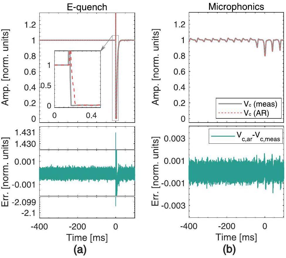
Further analyses were performed using the XGBoost model. We conducted a comprehensive analysis of the classification accuracy of the model for different categories using a confusion matrix. Confusion matrix analysis identifies a model's weaknesses, enabling targeted adjustments to parameters, feature engineering, and other aspects of model optimization. Figure 11 (left) shows that the XGBoost model based on AR features has a lower accuracy for faults such as E-quench, flashover, and microphonics, which may be attributed to the difficulty of the AR method in capturing the signal features of these three fault types. As shown in Fig. 12, the amplitude of Vc for E-quench exhibits significant abrupt changes, leading to substantial errors at the mutation positions when the AR method is employed to fit these signals. For continuously changing signals, such as microphonics, the AR method can capture data trends. However, this trend may be insufficient to describe microphonics fault features, thereby reducing the accuracy of the model in identifying microphonics faults.
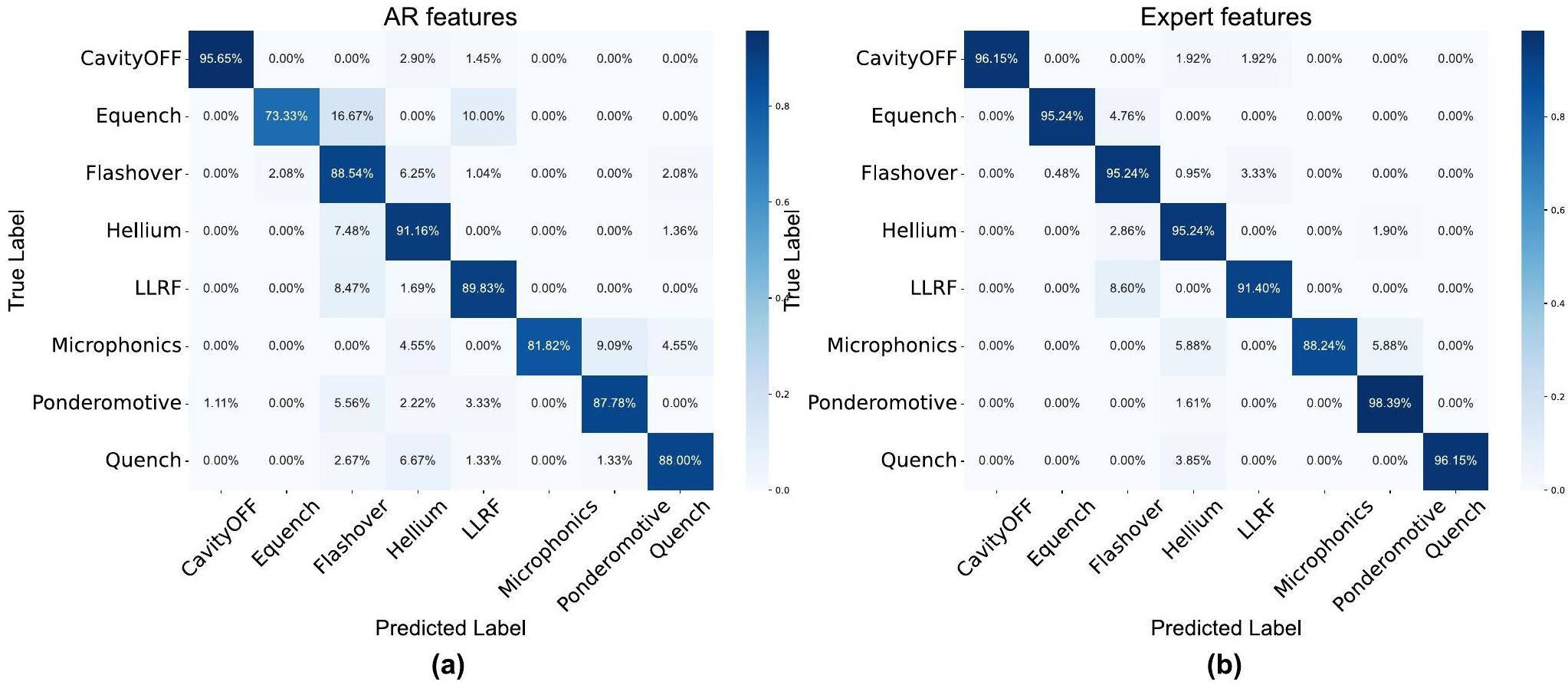
As displayed in Fig. 11 (right), the expert feature–based XGBoost model effectively addresses the challenges associated with the AR method. The introduction of expert features increases the accuracy of the model in capturing essential task-related features, thereby enhancing its applicability and performance. Subsequently, we interpreted the reasons for the improvement in the performance of the model from the perspective of feature importance analysis.
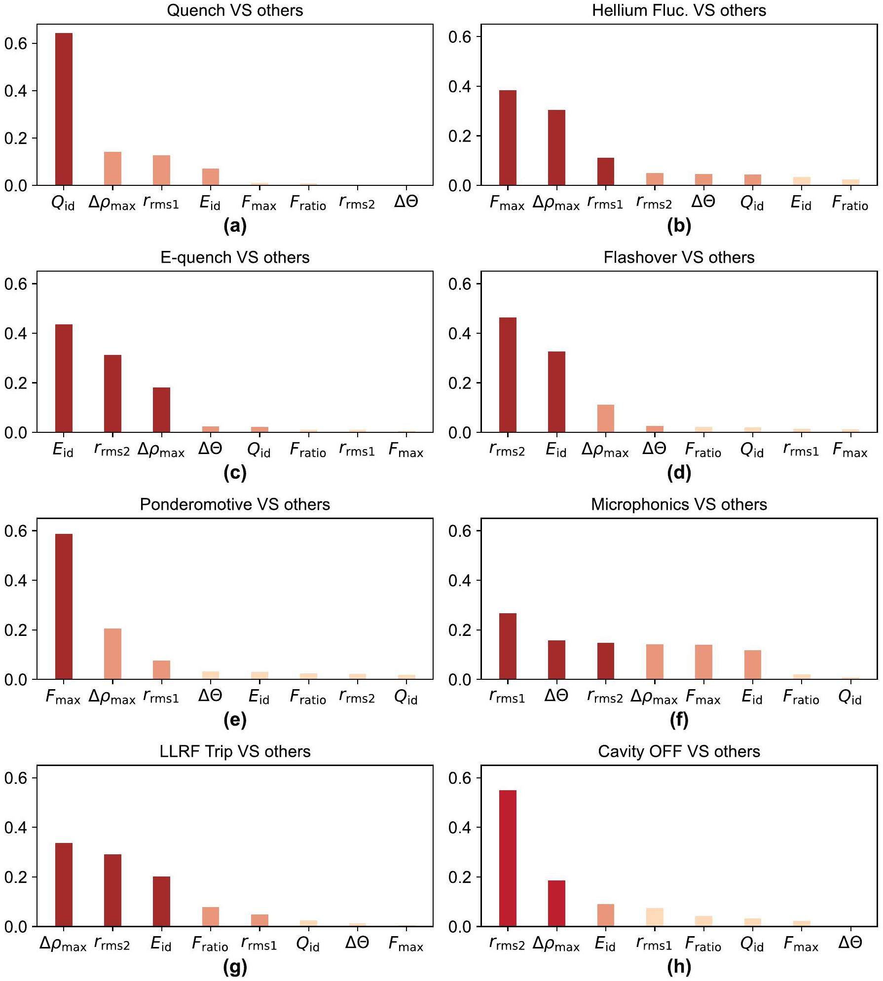
First, the multiclass problem was transformed into a binary classification problem, after which the information gain was utilized as a measure of the contribution of each feature to the model's predictions. As shown in Fig. 13, during the identification of the quench fault, the Qid feature exhibits the highest contribution. For the recognition of ponderomotive and helium faults, the Fmax feature was the most influential. For E-quench fault identification, the Eid feature exhibits the highest contribution. This indicates that the optimal segmentation features selected by the XGBoost model based on information gain align with the reasoning process adopted by experts during the fault analysis. Furthermore, various feature combinations have been used in the identification process for each fault, particularly for microphonics faults, which pose a major challenge for control room operators. The significance of this study is substantiated in terms of rational feature engineering and model interpretability.
Big data analysis of cavity faults
The trained XGBoost model was employed to analyze the historical data generated by CAFE2 during its operation. The fault data for CAFE2's daily operations are packaged into zip files, each containing four folders that store the RF signals of the fault cavities in the four cryomodules (CM1–CM4). Each fault event is named as “cavity name” + “fault time” (accurate to microseconds). Algorithm 1 summarizes the workflow of the ML method for classifying offline fault events. Notably, the output fault time, cavity name, and fault type can be used in future collective fault analyses.
| Initialization: | |
| Import relevant libraries in Python | |
| Load trained XGBoost model | |
| Obtain all fault data (N) | |
| Input: a csv file | |
| Output: fault time, cavity name, fault type | |
| for i in range(N) do | |
| data, fault time, cavity name Load file(i) | |
| Vc, Vf, Vr ←Preprocess data(data) | |
| features ← Extract features(Vc, Vf, Vr) | |
| fault type = Predict fault(features, model) | |
| end for | |
Using the ML model based on fault data from the second half of 2023, the probability of faults for a given pattern occurring in each cavity was calculated, as shown in Fig. 14, where the cavities prone to faults in this particular pattern are highlighted. The histograms reveal that the results of the AR-based and expert feature-based models were generally consistent when analyzing historical big data. Notably, the statistical results for E-quench (Fig. 14c and microphonics (Fig. 14f) faults, the AR model identified CM3-5 as prone to E-quench and CM4-1 as prone to microphonics. After verification, the expert feature-based method classified these faults as Flashover or helium, with subtle differences observed in the corresponding cavities in Fig. 14d and 14b. Subsequently, we consulted the fault data with subject-matter experts, and their assessments concurred with the inferences made by the expert feature-based model. These findings further substantiate the generalization capability of the proposed method. Moreover, the statistical results of the AR feature based model serve as a comparative baseline, offering an alternative perspective that reinforces the robustness of our conclusions.
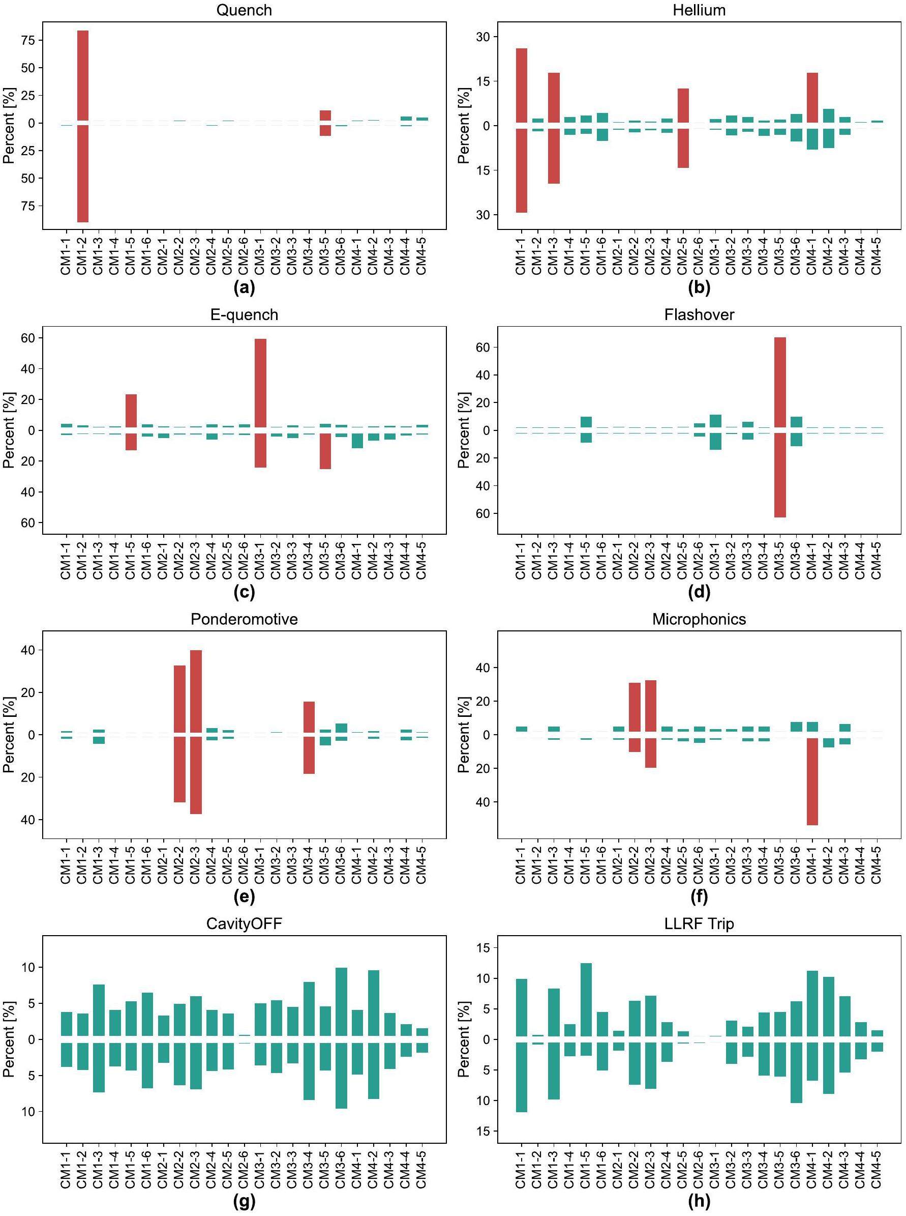
As shown in Fig. 14e and 14f, CM2-2 and CM2-3 are susceptible to vibration-induced microphonics and ponderomotive faults. In the subsequent operations, we increased the loop gain of the low-level system corresponding to CM2-2 and CM2-3. CM1-5, CM3-1, and CM1-2 were identified as the primary sources of E-quench and quench faults; we will reduce the acceleration gradient of these cavities in subsequent operations. In conclusion, employing ML for big data analysis is of great significance for enabling system experts to quickly identify the sources of faults and ensure the stable operation of accelerators.
Experience for feature engineering
This study provides a summary of fault types occurring in SRF cavities operating in the CW mode, along with discussions on fault mechanisms and feature engineering methods. Although the specific faults in SRF cavities may vary across different accelerators, there are similarities in the waveforms. Therefore, the feature engineering techniques proposed in this study offer valuable insights into the detection of faults in the SRF community.
1. For quench and helium faults, quantities such as Qid and
2. For vibration-related faults, such as ponderomotive and microphonics faults, methods such as FFT and wavelet transforms can be employed to extract the main vibration frequency and its corresponding energy.
3. For faults involving transient changes, such as E-quench, flashover, and LLRF trips, the first-order difference can be utilized to extract abrupt change values.
4. Some statistical features, such as the root-mean-square radius (e.g., rrms1 and rrms2), peak-to-peak value, and waveform factor can be used to describe the shape features of the waveforms.
These insights are valuable for the SRF community and aid in the development of fault detection and analysis techniques across various accelerators.
Future work
Based on our expertise and ML methods, we successfully classified the SC cavity faults. The next step in this study involves several potential expansions.
1. Use of deep learning (DL) methods instead of ML methods for fault classification. ML methods rely on feature engineering, encompassing both expert and AR features that are fixed and cannot be tuned during training. Therefore, we will explore DL models to build an end-to-end model structure that combines inference and feature representation learning, using raw waveform signals as inputs with simultaneous optimization via gradient backpropagation. DL requires numerous training samples. Nevertheless, the ML model and PCA method proposed in this study can provide ample and reliable labeled samples for DL, thereby reducing manual costs.
2. Research on fault prediction algorithms. In previous studies, we found that an SC cavity experiences an unhealthy state when transitioning from a healthy to a fault state. If anomalous states can be predicted in advance and inhibitory measures can be implemented, fault-induced accelerator downtime can be avoided. Therefore, another extension of this study involves exploiting DL algorithms for the early prediction of failures.
Summary and conclusion
We proposed an expert-feature-based automatic recognition method for CAFE2 SRF cavity faults. The confusion matrix and feature importance analyses indicated that the implemented feature engineering technique was reasonable and successful. Moreover, this method is not restricted by the sampling rate and performs excellently with data collected at sampling rates of 10–100 kHz.
ML, as a data-driven method, cannot be sufficiently emphasized because of its reliance on data. Each step is crucial, from data collection and labeling to feature extraction. Based on our experience, we suggest combining various data visualization methods, such as feature distribution analysis, PCA/TSNE analysis, unsupervised clustering, and information gain, to improve the quality of data labeling and the understanding of underlying patterns, thus increasing the accuracy of the ML model. Currently, this method only works offline; therefore, its importance lies in data analysis. During the beam commissioning process, the model can serve as a good assistant for controlling room operators. During the annual maintenance, the historical operation data analysis results provide valuable guidance for the maintenance and upgrading of SRF cavities.
Beam physics design of a superconducting linac
. Phys. Rev. Accel. Beams 37,Accelerator driven sustainable fission energy
, in Proceedings of the 7th International Particle Accelerator Conference,Transfer line including vacuum differential system for a high-power windowless target
. Phys. Rev. Accel. Beams 23,Physics design of the CIADS 25 MeV demo facility
. Nucl. Instrum. Meth. A 843, 11-17 (2017). https://doi.org/10.1016/j.nima.2016.10.055Operation experience at CAFe
, in Oral Presentation of the 2021 International Conference on RF Superconductivity, virtual conference, 2021. Available at https://indico.frib.msu.edu/event/38/attachments/160/1298/MOOFAV03_yuan_he.pdfInvestigation of decay modes of superheavy nuclei
. Nucl. Sci. Tech. 32, 130 (2021). https://doi.org/10.1007/s41365-021-00967-yCr-induced fusion reactions to synthesize superheavy elements, Nucl
. Sci. Tech. 35, 90 (2024). https://doi.org/10.1007/s41365-024-01449-7Discovery of new isotope 241U and systematic high-precision atomic mass measurements of neutron-rich Pa-Pu nuclei produced via multinucleon transfer reactions
. Phys. Rev. Lett 130,Discovery of new isotopes 160Os and 156W: revealing enhanced stability of the N=82 shell closure on the neutron-deficient side
. Phys. Rev. Lett 132,Predictions of the decay properties of the superheavy nuclei 293,294119 and 294,295120
(in Chinese). Nucl. Tech. 46,Development of the heavy ion RFQ for CAFE2
. Nucl. Instrum. Meth. A 1058,Results and perspectives for study of heavy and super-heavy nuclei and elements at IMP/CAS
. Eur. Phys. J. A. 58, 158 (2022). https://doi.org/10.1140/epja/s10050-022-00811-wA gas-filled recoil separator, SHANS2, at the China Accelerator Facility for Superheavy Elements
. Nucl. Instrum. Meth. A 1050,Multi-frequency point supported LLRF front-end for CiADS wide-bandwidth application
. Nucl. Sci. Tech. 31, 29 (2020). https://doi.org/10.1007/s41365-020-0733-9Design, fabrication and test of a taper-type half-wave superconducting cavity with the optimal beta of 0.15 at IMP
. Nucl. Eng. Technol. 52, 1777-1783 (2020). https://doi.org/10.1016/j.net.2020.01.014Development of a low beta half-wave superconducting cavity and its improvement from mechanical point of view
. Nucl. Instrum. Meth. A 953,Ultrahigh accelerating gradient and quality factor of CEPC 650 MHz superconducting radio-frequency cavity
. Nucl. Sci. Tech. 33, 125 (2022). https://doi.org/10.1007/s41365-022-01109-8Superconducting radio-frequency cavity fault classification using machine learning at Jefferson Laboratory
. Phys. Rev. Accel. Beams 11,Operational Availability of the SNS During Beam Commissioning
,Progress and experience at CAFe
, in oral presentation of 2021 International Conference on RF Superconductivity (SRF2021),Opportunities in Machine Learning for Particle Accelerators
, arXiv:1811.03172. https://arxiv.org/abs/1811.03172Orbit correction based on improved reinforcement learning algorithm
. Phys. Rev. Accel. Beams 26,Uncertainty aware deep learning for fault prediction using multivariate time series signals
,Improvements of pre-emptive identification of particle accelerator failures using binary classifiers and dimensionality reduction
. Nucl. Instrum. Meth. A 26,Fault locating for traveling-wave accelerators based on transmission line theory
. Nucl. Sci. Tech. 34, 116 (2023). https://doi.org/10.1007/s41365-023-01279-zA non-invasive diagnostic method of cavity detuning based on a convolutional neural network
. Nucl. Sci. Tech. 33, 94 (2022). https://doi.org/10.1007/s41365-022-01069-zAnomaly detection of control rod drive mechanism using long short-term memory-based autoencoder and extreme gradient boosting
. Nucl. Sci. Tech. 33, 127 (2022). https://doi.org/10.1007/s41365-022-01111-0Deep Learning Based Superconducting Radio-Frequency Cavity Fault Classification at Jefferson Laboratory
. Front. Artif. Intell. Appl. 4,CEBAF C100 Fault classification based on time domain RF signals
, in Proceedings of the 19th International Conference on RF Superconducting (SRF2019),A phenomenological model of the fundamental power coupler for a superconducting resonator
. Nucl. Sci. Tech. 34, 67 (2023). https://doi.org/10.1007/s41365-023-01215-1Application of a modified iterative learning control algorithm for superconducting radio-frequency cavities
. Nucl. Instrum. Meth. A 1026,Online detuning computation and quench detection for superconducting resonators
. IEEE T. on Nucl. Sci. 68, 385-393 (2021). https://doi.org/10.1109/TNS.2021.3067598Detection and suppression of the trapped-electrons-transportation-type flashover in a linear accelerator
. Phys. Scr. 96,Insitu Mitigation strategies for field emission-induced cavity faults using low-level radiofrequency system
. Nucl. Sci. Tech. 33, 140 (2022). https://doi.org/10.1007/s41365-022-01125-8Ponderomotive instabilities and microphonics—a tutorial
. Physica C: Superconductivity 441, 1-6 (2006). https://doi.org/10.1016/j.physc.2006.03.050An approach to characterize Lorentz force transfer function for superconducting cavities
. Nucl. Instrum. Meth. A 1012,Ponderomotive instability of Generator-Driven Cavity
, in Proceedings of the 10th International Particle Accelerator Conference,Anomaly detection at the European X-ray Free Electron Laser using a parity-space-based method
. Phys. Rev. Accel. Beams 26,Approach to calibrate actual cavity forward and reflected signals for continuous wave-operated cavities
. Nucl. Instrum. Meth. A 1034,Precise calibration of cavity forward and reflected signals using low-level radio-frequency system
. Nucl. Sci. Tech. 33, 4 (2022). https://doi.org/10.1007/s41365-022-00985-4Development of a finite state machine for the automated operation of the LLRF control at FLASH
,Superconducting cavity quench detection and prevention for the European XFEL
, in Proceedings of the 14th International Conference on Accelerator & Large Experimental Physics Control Systems,Measurement of the cavity-loaded quality factor in superconducting radio-frequency systems with mismatched source impedance
. Nucl. Sci. Tech. 34, 123 (2023). https://doi.org/10.1007/s41365-023-01281-5Ensemble-based classifiers
. Artif. Intell. Rev. 33, 1-39 (2010). https://doi.org/10.1007/s10462-009-9124-7Random forests
. Mach. Learn. 45, 5-32 (2001). https://doi.org/10.1023/A:1010933404324Bagging predictors
. Mach. Learn. 24, 123-140 (1996). https://doi.org/10.1023/A:1018054314350XGBoost: A Scalable Tree Boosting System
, in Proceedings of the 22nd ACM SIGKDD International Conference on Knowledge Discovery and Data Mining,Yuan He is an editorial board member for Nuclear Science and Techniques and was not involved in the editorial review, or the decision to publish this article. All authors declare that there are no competing interests.

