The three-body Gamow coupled-channel method

In this study, we focused on atomic nuclei that can be effectively described as three-body systems. Within the three-body GCC model, such systems are modeled as frozen cores with two valence nucleons. The corresponding Hamiltonian is given by $H(c)={\displaystyle \sum _{i=1}^3}\frac{p_i^2}{2m_i}+{\displaystyle \sum _{j=2}^3}{V}_{1j}^{\left[c_0\mathrm{,}{c}_1\right]}\left(r_{1j}\right)+c_2{V}_{23}\left(r_{23}\right)-T_{\text{c}\text{.m}\text{.}}\mathrm{,}$ (1) where the kinetic energy of each cluster is represented by $p_i^2/2m_i$ and $T_{\text{c}\text{.m}\text{.}}$ is the kinetic energy of the center of mass. The potential energy consists of the interactions between the clusters; specifically, $V_{1j}$ represents the nuclear force between the frozen core and each valence nucleon, which is modeled using the phenomenological Woods–Saxon (WS) potential within the GCC approach. The potential is expressed as follows: $V_{\text{W}S}^{\left[c_0\mathrm{,}{c}_1\right]}\left(r\right)=c_0\cdot V_{0}f(r)+c_1\cdot V_{\text{s}\text{.o}\text{.}}\left(\frac{1}{r}\frac{\text{d}}{\text{d}r}f(r)\right)\cdot \left(\overrightarrow{l}\cdot \overrightarrow{s}\right)+V_{\text{Coul}}\left(r\right)\mathrm{,}$ (2) where the form factor $f(r)$ is given by $f(r)=\frac{1}{1+\exp \left\{\left(r-R_{\mathrm{0,}\text{s}\mathrm{.}\text{o}\mathrm{.}}\right)/a\right\}}\mathrm{.}$ (3) In addition, the Coulomb potential is defined by the point-charge formula when the distance between two clusters exceeds the Coulomb radius R_C, while transitioning to a finite-distribution form when the distance becomes smaller than R_C.

The nucleon-nucleon interaction between the two valence nucleons $V_{23}\left(r_{23}\right)$ was modeled using the Minnesota potential [37]. To capture the different effects of the nuclear force and ‘pairing’ interactions, we introduce a set of three potential strength parameters, $c={\left[c_0\mathrm{,}{c}_1\mathrm{,}{c}_2\right]}^{\text{T}}$. Specifically, c₀ governs the central potential, c₁ accounts for spin-orbit coupling, and c₂ indicates the nucleon-nucleon interaction. These parameters set the stage for exploring how non-affine parameters influence the entire potential, thereby providing a framework for future investigations.

In the GCC framework, the total three-body wave function is expressed in Jacobi coordinates, which is particularly advantageous for describing the asymptotic behavior of the system [33, 38]. The angular components are constructed using hyperspherical-harmonic oscillator basis functions, while the radial part—determined by a set of quantum numbers representing various configurations—is expanded using the Berggren basis [39, 40]. This basis is directly related to the incoming and outgoing momenta of free particles as well as the complex energy of the eigenstates, satisfying the orthogonality and completeness relationship [41]. The Berggren basis is a key feature of the GCC model, allowing it to treat scattering states, resonances, and bound states equally. This provides a universal framework for modeling the nuclear structure and scattering properties.

Bayesian inference framework

The basic philosophy of Bayesian inference is encapsulated by Bayes’ theorem, which in this context is expressed as: $P(c|E)=\frac{P(E|c)\times P(c)}{P(E)}\mathrm{,}$ (4) where $P(c|E)$ is the posterior probability that represents the updated distribution of model parameters c after incorporating the observed data E. The term $P(E|c)$ is the likelihood, which describes the probability of observing data E given the parameters c. P(c) represents the prior probability that encodes the initial belief regarding the parameters before observing any data. The denominator $P(E)$ is the marginal likelihood, which ensures that the posterior sums to one. Therefore, the key function in Bayesian inference is $posterior\propto likelihood\times prior\mathrm{.}$ (5) In this study, we applied a Bayesian framework to quantify uncertainties in the three-body energy and the associated sensitivities of the strength parameters for nuclear and nucleon-nucleon forces between valence pairs. We assume that the error between the observable energy and model predictions follows a normal distribution; therefore, the likelihood is expressed as Gaussian: $\begin{array}{l}P(E|c)=\frac{1}{\sqrt{2\pi {\sigma }_{\text{R}}^2}\sqrt{2\pi {\sigma }_{\text{I}}^2}}\\ \times \exp \left\{-\frac{1}{2}\left[{\left(\frac{y{\left(c\right)}_{\text{R}}-E_{\text{R}}}{{\sigma }_{\text{R}}}\right)}^2+{\left(\frac{y{\left(c\right)}_{\text{I}}-E_{\text{I}}}{{\sigma }_{\text{I}}}\right)}^2\right]\right\}\mathrm{,}\end{array}$ (6) where y(c) is the energy predicted by the model for parameters 𝒄 and E_R,I are the real and imaginary components of the observed energy, respectively, and σ_{R, I} represents the experimental errors in the real and imaginary parts, respectively. The error $E_{\text{R}\mathrm{,}\text{I}}=y{\left(c\right)}_{\text{R}\mathrm{,}\text{I}}+{ϵ}_{\text{R}\mathrm{,}\text{I}}$ consists of three components: intrinsic model error (${ϵ}_{\text{R}\mathrm{,}\text{I}}^{\text{mo}}$), emulator error (${ϵ}_{\text{R}\mathrm{,}\text{I}}^{\text{em}}$), and experimental error (${ϵ}_{\text{R}\mathrm{,}\text{I}}^{\text{ex}}$). Each of these errors follows a normal distribution with standard deviations ${\sigma }_{\text{R}\mathrm{,}\text{I}}^{\text{mo}}\mathrm{,}{\sigma }_{\text{R}\mathrm{,}\text{I}}^{\text{em}}$, and ${\sigma }_{\text{R}\mathrm{,}\text{I}}^{\text{ex}}$, respectively. These contribute to the total error, which is given by ${\sigma }_{\text{R}\mathrm{,}\text{I}}^2={\left({\sigma }_{\text{R}\mathrm{,}\text{I}}^{\text{mo}}\right)}^2+{\left({\sigma }_{\text{R}\mathrm{,}\text{I}}^{\text{em}}\right)}^2+{\left({\sigma }_{\text{R}\mathrm{,}\text{I}}^{\text{ex}}\right)}^2\mathrm{.}$ (7) Next, we utilize Markov Chain Monte Carlo (MCMC) methods to sample from the posterior distribution. MCMC provides a way to avoid direct computation of the marginal likelihood $P(E)$, which would be computationally expensive. In each step, new parameter proposals are drawn from a normal distribution, and the acceptance probability is determined using the Metropolis algorithm. $\mathcal{A}(c\to c\text{'})=\text{min}\left(\mathrm{1,}\frac{p(c\text{'}|E)}{p(c|E)}\right)\mathrm{,}$ (8) where lowercase p is the posterior computed as the product of the likelihood and prior, and c and c' represent the current and proposed parameters, respectively. This approach satisfies the detailed balance condition, ensuring that the sampling distribution converges to the true posterior distribution.

However, the high computational cost of high-fidelity models, such as GCC, makes direct evaluations for every parameter sample prohibitive. To overcome this challenge, we employed an emulator based on the reduced-basis method, which offers a fast and accurate approximation of the original model. This emulator dramatically reduces the computational time while preserving the accuracy, thereby enabling efficient posterior sampling within a feasible timeframe.

The emulator

Intrinsically, the wavefunction exhibits several consistent properties as the parameters of the Hamiltonian in Eq. (1) vary, assuming that the system remains linear. For example, when the total potential strength 𝑽 is sufficiently large, the system becomes tightly bound and the corresponding eigenstate wave function is spatially localized. By contrast, for a weak total potential strength, the system becomes loosely bound or unbound, and the wave function displays an extended asymptotic tail, which is characteristic of resonant states [35]. By leveraging these properties, one can avoid repeated diagonalization of the high-dimensional, high-fidelity Hamiltonian in Eq. (1) for each parameter set. Instead, the emulator algorithm learns the trajectory of the wave functions across the parameter space, thereby enabling efficient and accurate predictions. This is mathematically expressed as ${\text{Ψ}}_{\odot }\approx {\displaystyle \sum _{n=0}^{N_b-1}}{a}_n{\text{Ψ}}_n^{\text{RB}}\mathrm{.}$ (9) Here, the wave function ${\text{Ψ}}_{\odot }$ of the target Hamiltonian, governed by specific parameters, is written as a linear combination of Nb reduced basis functions ${\text{Ψ}}_n^{\text{RB}}$. These reduced basis functions are generally chosen as high-fidelity solutions for selected parameters, which can be prepared in advance during the offline stage [42]. Numerically, we apply principal component analysis (PCA) to these high-fidelity solutions to extract the main features of the physical wave function, further reducing the number of required reduced basis functions [25]. We refer to the resulting reduced basis as the training basis because it captures the essential physical features of eigenstates.

This basis spans a low-dimensional subspace that effectively represents the main characteristics of the physical eigenstates, in stark contrast to the significantly larger dimensionality of the original free-particle basis. By inserting the reduced basis expansion into the Schrödinger equation, we obtain a projected Hamiltonian defined in this reduced subspace, with matrix elements given by ${\tilde{H}}_{mn}={\text{Ψ}}_m^{\text{RB}}{}^{*}\text{H}{\text{Ψ}}_n^{\text{RB}}\mathrm{,}$ (10) The associated norm matrix is defined as $N_{mn}={\text{Ψ}}_m^{\text{RB}}{}^{*}{\text{Ψ}}_n^{\text{RB}}\mathrm{.}$ (11) The approximated eigenstate $E_{\odot }$ was then determined as an eigenvalue of the combined matrices. The eigenvectors correspond to the solutions of the basis coefficients {an} in Eq. (9).

A central challenge in reduced-basis modeling is identifying the physically relevant eigenstate among many solutions of the reduced subspace. In contrast to high-fidelity calculations based on the Berggren basis—where the analytic structure of the complex energy plane facilitates clear classification of bound, resonant, and scattering states—the emulator’s eigenvalues are often irregularly distributed and do not exhibit distinct branch cuts. Consequently, additional selection criteria were required to isolate the target physical eigenstate.

One possible approach is to examine the eigenvector components on a principal-component basis. In theory, physically meaningful eigenstates should exhibit dominant contributions from the first few principal components, because these components are associated with localized structures in the configuration or momentum space. However, this strategy is hindered by the complexity of configuration mixing and the lack of direct physical interpretability of the individual principal components.

Given that the current reduced basis method (RBM) is mathematically equivalent to a variational approach [24], the physical eigenstate is expected to closely resemble the training basis. In contrast, spurious solutions—such as those corresponding to scattering-like states—typically show weaker projections onto this basis. To distinguish the target eigenstate robustly, we adopted an overlap-based method. In this approach, a reference wave function is selected in advance, and the overlap between this reference and each eigenfunction in the reduced subspace is computed as: $\text{Overlap}(i)=\left|{\text{Ψ}}_{\text{ref}}^T{\text{Ψ}}_i\right|\mathrm{,}$ (12) where ${\text{Ψ}}_i$ represents the i-th eigenvalue solution in the subspace and ${\text{Ψ}}_{\text{ref}}$ is the reference. The maximum overlap indicates the solution corresponding to the target state.

To improve the accuracy of the emulator’s approximation, we applied a wavefunction correction scheme inspired by the Lippmann–Schwinger equation [43] using the following iterative formula: ${\text{Ψ}}_{\odot }^{\left(i+1\right)}=\omega \cdot \frac{\text{V}{\text{Ψ}}_{\odot }^{\left(i\right)}}{E_{\odot }^{\left(i\right)}-\text{diag}\left(E_0\right)}+(1-\omega )\cdot {\text{Ψ}}_{\odot }^{\left(i\right)}\mathrm{.}$ (13) where ω is a relaxation factor used to preserve the local features of the initial emulator solution and suppress divergence toward scattering-like solutions. Once the corrected wave function is obtained, the energy is updated as $E_{\odot }^{\left(i+1\right)}={\text{Ψ}}_{\odot }^{\left(i+1\right)*}H{\text{Ψ}}_{\odot }^{\left(i+1\right)}\mathrm{,}$ (14) While a more detailed analysis of the L–S correction method is provided in [43], the present work focuses on its preliminary performance and its effectiveness in improving emulator predictions for realistic physical systems.

Model space and parameters

We selected the two-proton emitter ⁶Be as our test nucleus, which has been extensively studied [44-46]. The experimental energy of the 0⁺ state of ⁶Be has been reported to be 1.372 - 0.092i MeV.

In the GCC framework, the hyperangular configuration for ⁶Be is constructed as described in Ref. [33]. The quantum number set $\left(K\mathrm{,}{\mathcal{l}}_x\mathrm{,}{\mathcal{l}}_y\right)$ determines the different configurations, where we set $\max \left({\mathcal{l}}_x\mathrm{,}{\mathcal{l}}_y\right)\le 8$ and $K_{\max }=16$. We employ the Berggren basis for channels, where $K_{\max }\le 3$ to account for continuum effects, using the Harmonic Oscillator (HO) basis with an oscillator length b = 1.75 fm and $N_{\max }=20$, supplemented in higher orbitals. Although the L–S correction method is theoretically inapplicable on an HO basis, we set the maximum hyperspherical quantum number $K_{\max }=8$ and used the Berggren basis for all angular parts.

To fit the experimental energy, we adjusted several nonaffine potential parameters and the Berggren basis contour. The nuclear force is primarily governed by six parameters, which we set as: $a=0.65\text{fm}$, $V_0=-49\text{MeV}$, $R_0=2\text{fm}$, $V_{\text{s}\text{.o}\text{.}}=30\text{MeV}$, $R_{\text{s}\text{.o}\text{.}}=2\text{fm}$, and the radius of the Coulomb potential R_C = 2 fm. The complex momentum Berggren basis contour is defined as $\tilde{k}=0\to 0.3-0.1i\to 0.4-0.05i\to 0.5\to 0.8\to 1.2\to 2\to 4\to 6$ (all in fm^-1), with 30 discretized scattering states in each segment. The nucleon-nucleon interaction was modeled using the Minnesota potential, with detailed parameters set as in Ref. [37].

To maximize the accuracy of the emulator, both the bound and resonance states were included in the training subspace, although the target state was resonant. The training parameter is the strength of the total potential, which varies between [0.9, 1] for resonance states and [1.2, 2] for bound states, to obtain their corresponding wave functions. PCA is then performed on the 20 training vectors with a singular value accuracy of 10^-15, which is close to the computational limitations of our current servers.

The standard deviation σ^mo was chosen empirically to ensure effective convergence of the probability distribution following previous studies, and was set to 0.25% of the corresponding experimental value [19, 27]. The error σ^ex is negligible compared with the other sources of uncertainty. For the emulator error σ^em, we collected random samples and fitted their error distribution with a Gaussian function as well as the Berggren basis contour properties, ultimately determining its value to be 15% of the experimental value, as will be discussed in detail later. Prior studies employed uncertainty decomposition methods to address model deviations with improved precision [7]. However, given the much larger deviations in our emulator, we omitted such corrections from this analysis.

We assume that the prior distribution for parameter vector 𝒄 follows a multivariate normal distribution as follows: $\left[\begin{array}{c}{c}_0\\ c_1\\ c_2\end{array}\right]\sim \mathcal{N}\left(\left[\begin{array}{c}1\\ 1\\ 1\end{array}\right]\mathrm{,}\left[\begin{array}{ccc}{0.25}^2& 0& 0\\ 0& {0.25}^2& 0\\ 0& 0& {0.25}^2\end{array}\right]\right)\mathrm{.}$ For each step in the Metropolis algorithm, new parameters were proposed using a multivariate Gaussian distribution, with the current parameter being the mean value. To ensure faster convergence, we adjusted the standard deviation to maintain an acceptance rate of approximately 30%~40% [47], setting it to 0.02·c.

Computational Performance of the Emulator

PCA is a powerful dimensionality-reduction technique that is particularly effective when the training space exhibits redundancy. To quantitatively assess this redundancy, we analyzed the singular values of the principal components and determined an appropriate cutoff for the subspace dimension. Fig. 1 shows the singular value spectrum of the dataset. Although resonance states feature abrupt changes in their asymptotic behavior compared with bound states, their key features can still be efficiently captured via PCA owing to similarities in the local structure of their wave functions. Specifically, the first component that captures the largest singular value in Fig. 1 resembles the shapes of the bound states. The second component corresponds to the average shape of a sharp peak in the resonance wave function in momentum space, as well as the oscillatory outgoing wave. The exponentially decaying weighted components are more similar to the free-particle basis, which is analogous to the Berggren basis.

Fig. 1Full-screen View

Singular values of the wave function distribution. n denotes the index of the principal components, and s represents their corresponding singular values

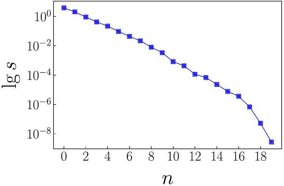
The singular value analysis indicates that our training space sufficiently captures the high-fidelity properties. While both bound and resonance features are included, the emulation process primarily functions as an interpolation operator because the parameter variations are smooth. Therefore, it is more reasonable to estimate the error between the emulator and GCC using a statistical approach rather than providing σ^em point by point.

As discussed previously, isolating the target eigenstate within the emulator subspace is crucial. To achieve this, we employed an overlap technique, which is mathematically defined in Eq. (12). Figure 2 presents the overlap analysis for a representative parameter point given by [c₀, c₁, c₂]^T = [0.9, 0.8, 1.1]^T. In this case, the reference wave function was chosen as the resonance state obtained using all potential strengths set to unity. This reference is sufficiently diffuse to suppress spurious overlaps with scattering-like states, which may otherwise introduce significant noise into the overlap calculation.

Fig. 2Full-screen View

Overlap between the reference state and eigenstates for the chosen parameters. The darkest and largest point represents the largest overlap, corresponding to the emulated eigenstate energy. The red square marks the exact energy calculated by GCC

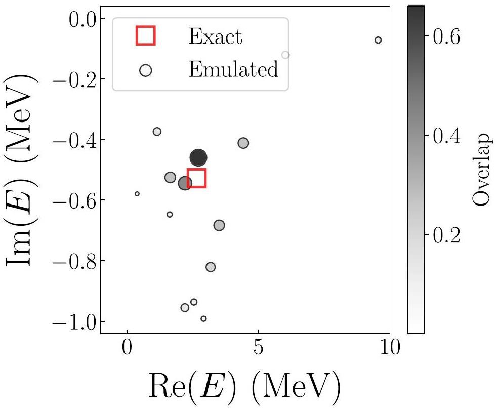
In Fig. 2, each circle corresponds to the eigenvalue of the emulator Hamiltonian in the reduced subspace. The size and color intensity of the circles represent the magnitude of overlap with the reference wave function. The largest overlap is associated with the emulator-predicted eigenstate, marked by the darkest circle, which yields an energy of $E_{\text{em}}=2.715-0.45(9)i$ MeV. For comparison, the exact result obtained from the full GCC model is $E_{\text{GCC}}=2.649-0.52(7)i$ MeV, shown as a red square. The non-negligible difference between these values highlights the necessity of incorporating emulator error into MCMC sampling to ensure a reasonable acceptance rate.

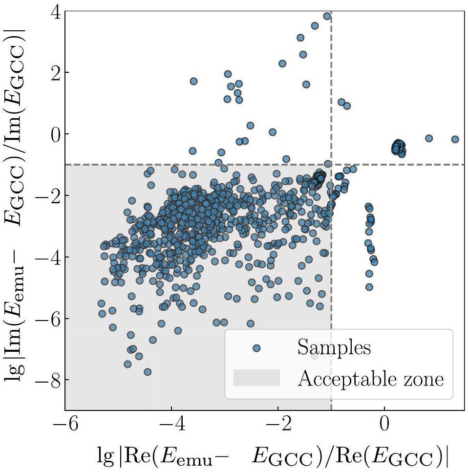
Assuming that the emulator error follows a normal distribution, we estimated it by sampling 1000 random parameter points. After excluding unphysical scattering-like states (102 invalid cases), we retained 898 valid samples for the analysis. The resulting relative error distributions are shown in Fig. 3, where over 90% of the predictions exhibited deviations below 10% in both the real and imaginary parts. The mean relative error is approximately 15%, demonstrating the overall robustness of the emulator. Relative errors provide a more consistent metric across varying energy scales than absolute deviations. In practice, because exact GCC results are unavailable during sampling, we use the experimental energy $E_{\text{exp}}$ as a practical reference for converting relative errors into absolute uncertainty, assigning ${\sigma }^{\text{em}}=15\%\cdot E_{\text{exp}}$. This threshold also serves to filter non-resonant or deeply bound states during posterior inference. While approximately 10% of the points exceed our acceptable error range, likely owing to pathological parameter configurations or model limitations, these outliers exhibit limited deviation magnitudes and negligibly impact our overall uncertainty estimates. The physical reasonableness of our results is further confirmed by the posterior energy distributions shown in Fig. 5, thus validating the uncertainty quantification approach.

Fig. 3Full-screen View

(Color online) Cross-validation of the emulator performance. The two axes show the log-scaled relative errors of the real and imaginary parts of the predicted energies, respectively. Dashed lines indicate the upper limit of the acceptable region, corresponding to a relative error of 10%

The remarkable computational efficiency of the emulator is worth emphasizing. The diagonalization of the projected Hamiltonian requires only 5.26 × 10^-3 s, which is nearly four orders of magnitude faster than the 36.6 s required for full high-fidelity GCC calculation. This acceleration enabled the use of an emulator for large-scale posterior sampling and uncertainty quantification.

Constraining potentials in ⁶Be

We investigated the 0⁺ ground state of ⁶Be by using our Bayesian analysis framework. Following a burn-in of 1,000 points and collection of 100,000 posterior samples, we achieved an acceptance rate of 36.7%. The entire computation was completed in approximately 3 h on a server, which would have required nearly four months without the use of the emulator.

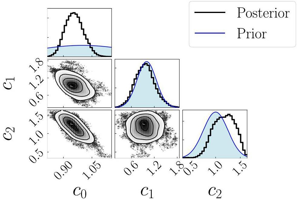
Figure 4 presents the posterior distributions for all three model parameters. Evidently, the central force strength c₀ is strongly constrained by the data. In contrast, the spin-orbit strength c₁ retains a distribution shape close to its prior value, suggesting limited sensitivity of the observable to this parameter in the current setting. The distribution of the nucleon-nucleon interaction strength c₂ shows a moderate deviation from the prior value, which may be attributed to a negative correlation with the central force strength c₀.

Fig. 4Full-screen View

(Color online) Posterior distributions of the parameters. c₀, c₁, and c₂ represent the strengths of the central force, spin-orbit coupling, and nucleon-nucleon interaction, respectively. The black histograms show the posterior distributions, and the blue curves represent the prior sampling regions

We further visualize the distribution of the calculated resonance energies under the sampled posterior parameters, as shown in Fig. 5. The peak values of the distributions exhibited noticeable deviations from the experimental resonance energies. This discrepancy may arise partly because the likelihood function is more sensitive to the imaginary part of energy, which is smaller than the real energy. Moreover, latent variables that are not directly sampled in this study, such as the diffuseness and radius parameters of the WS potential, also contribute to the overall model uncertainty.

Fig. 5Full-screen View

(Color online) Energy distribution of the posterior parameters. The blue histogram represents the real energy distribution, while the green histogram corresponds to the imaginary energy distribution. Each distribution has been fitted with a Gaussian function, with the mean value μ and standard deviation σ indicated

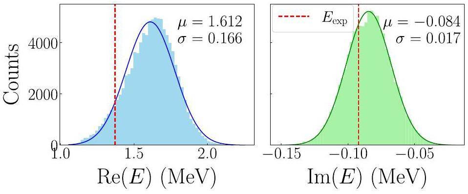
We fitted the predicted energy distributions shown in Fig. 5 to Gaussian functions, extracting both the mean (μ) and standard deviation (σ) values, which are indicated in the upper-right corner of each subplot. The predicted mean energies deviate by 17% (real energy) and 8% (imaginary energy) from the reference values. The energy deviations fall within approximately ± 1σ credible intervals, demonstrating the statistical consistency between the results of the emulator and the expected uncertainty distribution. Furthermore, this implies that emulators can be developed for other non-affine parameters in the future to investigate the overall impact of our model on multi-nucleon decay.

Correcting the emulated eigen-pair with L–S method

As discussed above, the (L–S) correction not only yields consistent improvements in both eigenvalues and wavefunctions, but also enables a natural extension of real-space training data to the complex energy plane.

Here, we examine the performance of our L–S correction method for two types of training spaces in the ⁶Be system: one composed of bound-state solutions, and the other of resonance-state solutions. We selected a representative parameter point, [c₀, c₁, c₂] = [0.925, 1,1.4], drawn from the posterior distribution shown in Fig. 4. This parameter set corresponds to a resonance state that is close to the experimental value.

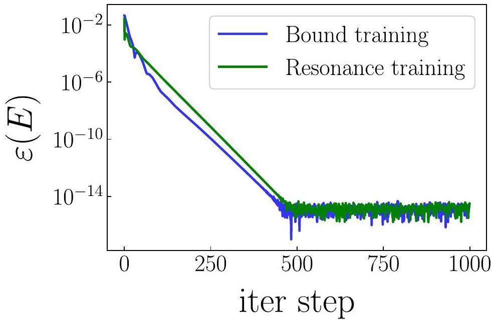
The maximum iteration step was set to 1000, and we defined ϵ(E) as the relative error of each step compared to the previous step. Figure 6 illustrates the convergence behavior of our iteration, whereas Table 1 lists the final corrected energy with high accuracy. The results demonstrate that the L–S correction can converge to nearly the same energy within a few hundred steps regardless of whether the training space consists of bound or resonance states. This is particularly beneficial for improving the extrapolation capability of the RBM, particularly when only bound high-fidelity solutions are available as a training subspace. In Table 1, the L–S correction significantly improved the energy accuracy, particularly the width, bringing it closer to the GCC high-fidelity value.

Fig. 6Full-screen View

(Color online) Convergence behavior of the L–S correction. The blue line represents the result when the RBM training space is constructed with bound states, where the total potential strength ranges from 2 to 2.5. The green line corresponds to the case where the training space is constructed with resonances, with the total potential strength ranging from 0.9 to 1

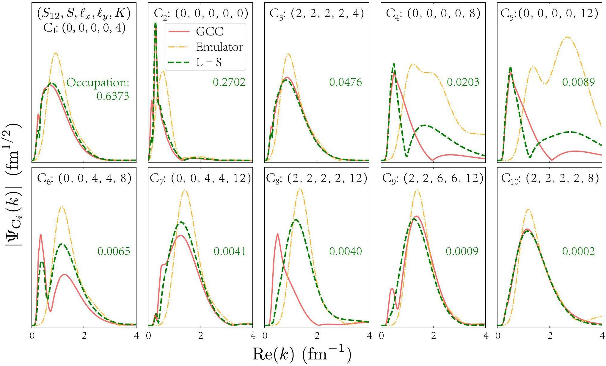
Remarkably, the L–S correction can restore the resonance energy even when the emulator subspace consists only of bound states, which do not exhibit oscillatory asymptotic behavior outside the nucleus in the resonance state. Fig. 7 illustrates how the wavefunction in momentum space is restored. The emulated wavefunction closely resembles that of the bound states, with small contributions from the low-momentum components and outer regions of the coordinate space. The dominant configurations, such as C₁ and C₂ with occupation probabilities exceeding 0.1 and quantum numbers K = 0 or 4, are well recovered, leading to an energy correction that closely approaches the resonance state. In contrast, configurations associated with higher K values (e.g., K = 8 and 12) exhibit larger deviations in the wavefunction shape compared with the high-fidelity results. These discrepancies are particularly pronounced at low momenta, particularly below 2 fm^-1. This can be attributed to the fact that high-K configurations typically represent the subdominant components in the total wavefunction. As such, infinitesimal features such as inflection points on the momentum axis, which are not well captured by the original emulator, can lead to amplified errors in the correction process. Nevertheless, these results highlight that the L–S correction method can be an effective tool for extending the emulator to continuum physics. Further studies should be conducted in the future.

Fig. 7Full-screen View

(Color online) Corrected wavefunctions for different configurations. Each configuration is labeled as ${\text{C}}_i$, where ‘i’ denotes integers from 1 to 10, ordered by decreasing occupation probability (shown as green numbers), respectively. Configurations are identified by the quantum numbers $\left(S_{12}\mathrm{,}S\mathrm{,}{\mathcal{l}}_x\mathrm{,}{\mathcal{l}}_y\mathrm{,}K\right)$. Each wavefunction is extracted from the total wavefunction and individually normalized to facilitate direct comparison