Introduction
Neutron time of flight facility n_TOF at CERN is a neutron production facility specializing in high-resolution measurements of the neutron induced reactions [1, 2]. In use since 2001, it is currently in the fourth major phase of its operation [3, 4]. Currently, it features three distinct experimental areas. The first and the second experimental area – EAR1 [2] and EAR2 [5-7] – are well established and have long since been in use. A new NEAR [8-10] experimental area is the most recent feature, characterizing the latest n_TOF phase.
The facility relies on a 20 GeV proton beam from the CERN Proton Synchrotron, which irradiates a massive Pb spallation target as a primary source of a neutron beam. The pulsed proton beam – 7 ns wide (RMS), with a minimum repetition period of 1.2 s – delivers an average of
Initially, fast spallation neutrons are moderated by passing through a spallation target itself, through a layer of demineralized water from a cooling system, and through an additional layer of borated water from a separate moderation system around the target. This yields a white neutron spectrum spanning more than 10 orders of magnitude in energy, from thermal (∼10 meV) up to ∼1 GeV (up to the order of magnitude, depending on the experimental area [11, 12]). The beam production, moderation, and transport mechanisms are well understood [13, 14].
An inevitable by-product of the neutron production and moderation is a finite spread of neutron arrival times at the measuring station from a given experimental area, even for the neutrons of the same kinetic energy. These arrival times are measured and treated as the neutron times of flight, relative to the single initial moment of the primary proton beam hitting the spallation target. There are three major effects causing the variations in times of flight: (1) a time width (7 ns RMS) of the primary proton beam; (2) a distribution of neutron moderation times inside the target-moderator assembly; (3) a geometry of neutron transport along the beamline of finite length and breadth. This spread in neutron arrival times gives rise to a distribution known as the resolution function of the neutron beam. It causes the smearing of the experimental spectra in the cross section measurements based on the time of flight technique. As such, it must be accounted for during the analysis of the experimental time of flight data. At n_TOF the resolution function considerations have been pursued ever since the initial conception of the facility [1] and continue to be followed since the start of its operation [15, 16] to the present day [2, 4, 5, 13, 14].
The only practical means of obtaining a detailed evaluation of the resolution function are the dedicated simulations of the neutron production and moderation. Because of the complexity of the target-moderator assembly at n_TOF, these simulations are so computationally intensive that their output needs additional post-processing by the so-called optical transport code [13, 14, 17]. The purpose of this code is to propagate the outgoing neutrons towards the measuring station and to refine the raw statistics from the primary simulations in a meaningful and computationally efficient way. However, the final output of this code is still subject to statistical fluctuations, which are detrimental to the quality of the experimental data analysis. Furthermore, the raw numerical format of the resolution function is rather cumbersome to deal with, requiring users to implement their own interpolation and smoothing procedures. For this reason, a smooth parametrization of the resolution function is highly desirable. A difficulty arises from the fact that the shape of the resolution function varies significantly over a wide energy range of the n_TOF beam, covering more than 10 orders of magnitude in neutron energy. Attempts have been made in the past to identify the appropriate analytical form, as in Ref. [2]. But this form is a rather complicated function of two variables: the neutron energy and the time of flight. As such, it is exceedingly difficult to identify, only to be invalidated after each modification of the neutron production system at n_TOF, for example, after the occasional upgrades of the spallation target, moderator assembly, beam collimation system, etc.
In this work, we present an efficient and streamlined method for a parametrization of the n_TOF resolution function by means of the machine learning techniques, together with a user-friendly interface for its evaluation. The interface consists of a dedicated C++ class centred around the neural network implementation from a widely used programming package ROOT [18]. As a proof of concept, we apply the methodology to the resolution function of the first experimental area (EAR1) from the third phase (Phase-3) of the n_TOF operation (2014–2018 [19, 20]; Phase-4 is in effect since 2021 [3, 19], after a long shutdown in 2019–2021). We disclose an optimal network structure for this particular resolution function, which should also serve as the optimal or near-optimal structure for its re-parametrization after any alteration of the resolution function, or even for the parametrization of a resolution function for a different experimental area. As such, a repeated neural network training procedure requires very little user input regarding a selection of the appropriate parametrization form (realized through a selection of hyperparameters defining a neural network structure).
Section 2 establishes a basic formalism behind the resolution function. Section 3 presents its parametrization by means of a trained neural network, together with a procedure for a numerical reconstruction of the various resolution function forms from a single parametrization. Section 4 summarizes the main conclusions of this work. The appendix addresses an apparent norm violation in applying the resolution function.
Resolution function formalism
A detailed resolution function formalism may be found in Ref. [21]. In this section, we summarize the most important points. For readability of expressions, we will use compact notations E and
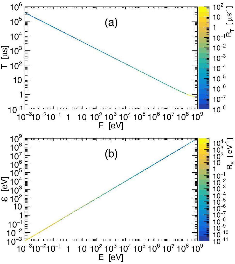
The other reason for a cumbersome nature of RT and
It should be noted that the effective moderation length λ is not the real path length of a neutron inside a spallation target, for multiple reasons: (1) a neutron inside a spallation target does not propagate the entire time with speed
Figure 2 shows a resolution function
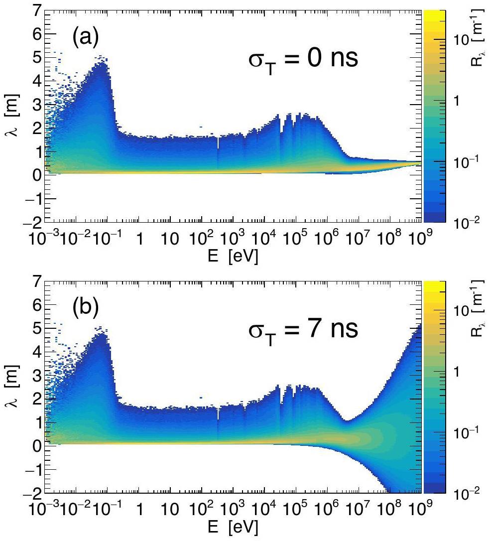
We now have a set of three kinematic parameters to be found in common use:
Resolution function parametrization by means of machine learning
Resolution function fitting
It was shown in Ref. [17] that the raw resolution function (obtained by the optical code) can not be used for a reliable resonance analysis. The reason is that the residual statistical fluctuations from the computationally intensive FLUKA+MNCP simulations of the neutron production and transport through the spallation target are not negligible relative to the fluctuations in the experimental data. Thus, using the raw resolution function in the analysis of the experimental data artificially and unnecessarily increases the involved statistical uncertainties. (Examples of smearing the initially smooth spectra by the raw resolution function may be found in later Figs. 5 and 6.) Clearly, a smoothed form of the resolution function is necessary, so as to avoid this adverse effect. It is also highly desirable that the smoothed form be efficiently parameterized, that is, that it is more compact than just a densely interpolated resolution function matrix filled with the values of a smoothed function (a matrix such as those from Figs. 1 and 2).
One way of proceeding would be to identify an analytical parametrization of the entire resolution function matrix. An example of such parametrization for a resolution function of EAR1 from Phase-1 of the n_TOF operation can be found in Ref. [2]. However, such an analytical form is difficult to identify and may no longer be appropriate when the alterations are introduced to the neutron production process. For example, the replacement of a spallation target between Phase-1 and Phase-2 of the n_TOF operation [4] notably affected the shape of a resolution function, rendering previous parametrization invalid. Furthermore, a resolution function for EAR2 differs from the one for EAR1 and requires its own dedicated parametrization. To avoid a tedious manual identification of new analytical forms, we take advantage of the machine learning techniques, in particular of the deep feedforward neural networks. The idea stems from a fact that the multilayer feedforward neural networks act as the universal approximators, capable of approximating any sufficiently well behaved function to any desired degree of accuracy [22, 23]. In other words, such networks can be thought of as “black box” fitting functions capable of modeling any function of practical importance. The application of neural networks to this task is a part of ongoing efforts to introduce the machine learning techniques into a widespread practice at n_TOF [24-26]. The possibility of applying the convolutional neural networks in unfolding the effects of the resolution function is also being investigated, with very promising results on the horizon [27].
We demonstrate the proof-of-concept by fitting a resolution function of EAR1, from Phase-3 of the n_TOF operation. To this end, we used the neural network training capabilities of the TMultiLayerPerceptron class [28] from root. Using root allows for a seamless integration of the end result (a trained neural network) within a vast majority of the data analysis codes from n_TOF. We provide a basic example of the code usage among the openly available data files [29].
Our goal is to fit a single form of a resolution function (either RT,
There is another consideration to be taken into account, that will allow for a greater flexibility in reconstructing particular forms of a resolution function. The resolution functions of the n_TOF facility (for different experimental areas) are affected by two separable contributions: (1) a neutron production and transport process inside a spallation target, as well as a neutron transport outside of it; and (2) a time distribution (a finite time width) of the primary proton beam from the CERN Proton Synchrotron irradiating the spallation target. The proton beam time distribution is Gaussian in shape with a standard deviation of σT=7 ns. Let
Here, we describe a neural network training and optimization procedure. First, the 450×60 numerical resolution function matrix was constructed, spanning 450 uniformly distributed λ values between -2 m and 7 m (2 cm steps), together with 60 isolethargically distributed
We tested several training methods available in the TMultiLayerPerceptron class, using a few preliminary network structures. We did not observe any significant improvement– either in the computational efficiency or in the quality of the final results – over the default Broyden-Fletcher-Goldfarb-Shanno (BFGS) method with the default hyperparameter values [28]. Hence, we opted for the default training parameters, employing the sigmoid activation function. In TMultiLayerPerceptron, the binary cross-entropy is the only loss function associated with the sigmoid activation function. By testing a range of network structures, we identified an optimal structure consisting of three hidden layers, each composed of 15 neurons. The optimal structure was easily identified. Less than three hidden layers do not seem to have enough flexibility to recover the quick variations in the resolution function, even with highly increased number of neurons. Aside from the visually obvious overfitting, more than three hidden layers do not bring any further improvement in the resolution function reconstruction. Once the optimal three-layer structure was identified, the number of neurons was varied in steps of five, in different combinations throughout the layers (e.g. 15-10-20). By searching for the simplest structure providing a satisfactory resolution function reconstruction – without further improvement with an increasing number of neutrons – we quickly converged upon the optimal 15-15-15 structure, which is shown in Fig. 3. The network inputs are
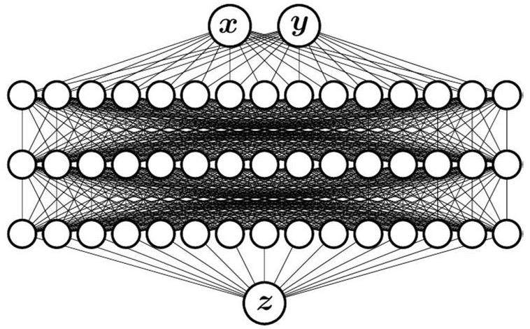
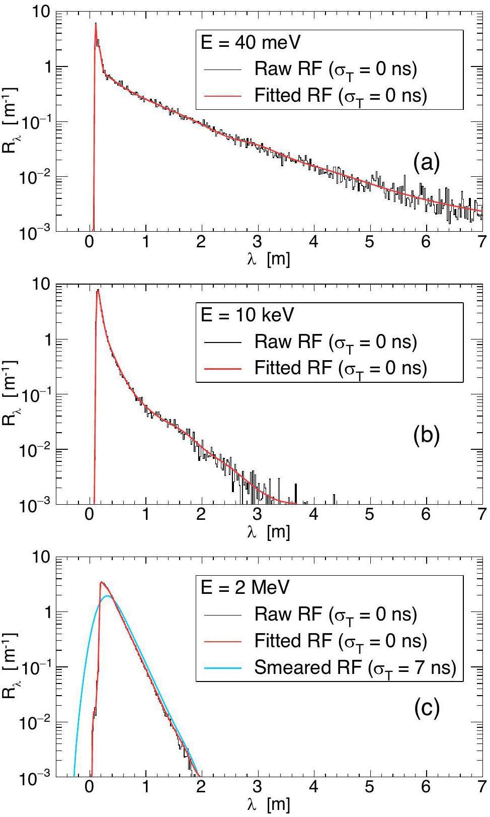
Figure 4 compares a raw resolution function with a fitted one, for several values of a true neutron energy E. The effect of a proton beam width is negligible below σλ=1 cm. As per Eq. (9), a time width of σT=7 ns implies an equivalent energy limit of E=10 keV (corresponding, for EAR1 flight path of L=180 m, to the times of flight below 0.13 ms). Hence, at lower neutron energies the proton beam width of 7 ns does not have any significant effect upon the resolution function. For this reason a resolution function smeared by means of a numerical convolution from Eq. (10) is shown only at energies higher than 10 keV.
Numerical resolution function reconstruction
To reconstruct the resolution function forms RT and
Because of a simple relation between λ and T from Eq. (4), a transformation rule for RT from Eq. (6) involves a very simple derivative Dλ/DT=vE, yielding:
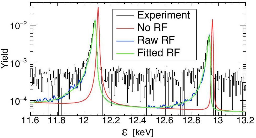
We use a transformed resolution function from Eq. (13) to demonstrate the effect upon and an agreement with the n_TOF experimental data. Figure 5 shows two selected resonances from a recent measurement of the 53Cr(n,γ) reaction in EAR1 [30]. Although the measurement was performed during n_TOF Phase-4, for presentation purposes, we use here a resolution function from Phase-3 as a first approximation of the resolution function from Phase-4. The plot shows a resolution-function-free reaction yield – manually constructed by appropriately scaling a neutron capture cross section from ENDF/B-VIII.0 database [31] – together with two resolution resolution-function-smeared yields, compared with the experimental data. (The preliminary experimental data are shown, as their analysis is not yet complete. The region between the resonances is still affected by the residual background contributions, not all of which have yet been subtracted. The relative background contribution inside the resonances is negligible for visual purposes, so that a meaningful visual comparison with the ENDF resonances can still be made.) Smeared yields have been obtained either by applying the raw, unparameterized resolution function or the one fitted by the neural network. Reaction yields (Y) transform precisely as the differential spectra from Eq. (7) and have been obtained by a transformation:
A simple and comprehensive insight into effects of applying either the raw or the smoothed resolution function may be obtained by applying them to a constant spectrum of unit height. Figure 6 shows these results for the
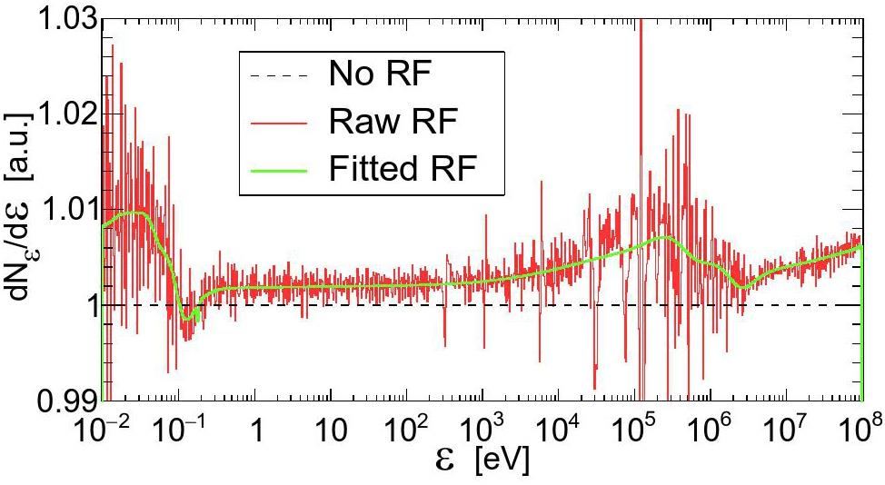
The resolution function affected spectra from Fig. 6 seem to be systematically higher than unity. This might suggest that the application of a resolution function violates a norm preservation, that is, it violates a conservation of the total number of underlying counts. This violation is only apparent and is addressed in the Appendix.
Resolution function class
To facilitate the use of a newly fitted resolution function at n_TOF, we have written a self-contained C++ class [35], serving as a simple interface for the evaluation of any desired resolution function form (Rλ, RT or
(1) initialization of a trained neural network (
(2) numerical normalization (
(3) smearing due to a proton beam width (
(4) transformation to alternative forms (
(5) computationally efficient implementation of the above operations.
The class houses the parameters of a trained neural network and initializes a TMultiLayerPerceptron object, allowing for a direct evaluation of a fitted, proton-beam-width-free (unnormalized) resolution function
In evaluating any form of a resolution function, the first operation to be performed is a numerical normalization such that
For a user-supplied value of a temporal proton beam width σT, a normalized resolution function Rλ is smeared by performing a discrete version of a convolution from Eq. (10). This is the most significant bottle-neck of the numerical calculations, since a naive convolution algorithm is computationally expensive. When users request single points of a resolution function (one point at a time), little can be done to speed up a convolution algorithm itself. In this case, our class offers a possibility of a bilinear interpolation, which will soon be described. However, significant algorithmic improvements are available when a convolution needs to be calculated (i.e. smearing needs to be performed) over a grid of uniformly spaced λ-points. While a naive convolution algorithm is of excessive
Having thus obtained a smeared Rλ, only a kinematic parameter transformation from Eq. (12) or (13) remains to be performed whenever the resolution function forms RT or
Conclusion
We have provided an efficient way of parametrizing a resolution function of a neutron beam from the n_TOF facility, thus solving a long-standing problem of facilitating its use among the users requiring a resolution function in their data analyses. The method takes advantage of the machine learning techniques. Specifically, the resolution function is fitted by training a multilayer feedforward neural network, due to the fact that such networks act as the universal approximators. We have applied the method to the resolution function for the first experimental area of the n_TOF facility, from the third phase of its operation. In order to re-parametrize the resolution function after any alteration – or to parametrize a resolution function for a different experimental area – one only needs to retrain a neural network by using the readily available streamlined procedures. In this work, we have used the neural network training capabilities of the TMultiLayerPerceptron class from a C++ based programming package root.
We have parametrized a single most appropriate form of the resolution function – one dependent on the so-called effective neutron-moderation length, and unaffected by the temporal spread of the primary proton beam from a neutron production process at n_TOF. To efficiently reconstruct several other resolution function forms in common use – those dependent on the neutron time of flight or the so-called reconstructed neutron energy – and to apply the effects of the proton beam width, we have supplied a specialized C++ class. The class is immediately applicable to any reparameterization of the resolution function, as the involved reconstruction procedures are independent of the underlying network structure. We have applied a reconstructed resolution function to the pre-established neutron capture resonances in the 53Cr(n,γ) reaction. We found an excellent agreement with the preliminary experimental data from n_TOF, thus providing a proof of concept that the resolution function parametrization proposed here is indeed feasible.
Unlike the resolution function for the first experimental area (EAR1) of the n_TOF facility, the one for the second experimental area (EAR2) features a strong nontrivial dependence on the sample position, that is, the distance from a neutron source (a Pb spallation target). Therefore, one could parametrize several separate EAR2 resolution functions at different sample positions of interest. On the other hand, a parametrization procedure proposed here could be easily extended so as to include a sample position as an additional input parameter, alongside a true neutron energy and an effective neutron-moderation length. By extending (reoptimizing) the network structure, a comprehensive parametrization of the EAR2 resolution function – particularly its variation along the neutron beam – could be achieved in a single go, for a wide range of sample positions.
A high resolution spallation driven facility at the CERN-PS to measure neutron cross sections in the interval from 1 eV to 250 MeV. (CERN/LHC/98-02 and CERN/LHC/98-02-Add.1, 1998)
, https://cds.cern.ch/record/363828. AccessedPerformance of the neutron time-of-flight facility n_TOF at CERN
. Eur. Phys. J. A 49, 27 (2013). https://doi.org/10.1140/epja/i2013-13027-6Status report of the n_TOF facility after the 2nd CERN long shutdown period
. EPJ Tech. Instrum. 10, 13 (2023). https://doi.org/10.1140/epjti/s40485-023-00100-wDesign of the third-generation lead-based neutron spallation target for the neutron time-of-flight facility at CERN
. Phys. Rev. Accel. Beams 24,The new vertical neutron beam line at the CERN n_TOF facility design and outlook on the performance
. Nucl. Instrum. Methods Phys. Res. A 799, 90-98 (2015). https://doi.org/10.1016/j.nima.2015.07.027The Second Beam-Line and Experimental Area at n_TOF: A New Opportunity for Challenging Neutron Measurements at CERN
. Nucl. Phys. News 25(4) 19-23 (2015). https://doi.org/10.1080/10619127.2015.1035930Optimization of n_TOF-EAR2 using FLUKA
. J. Instrum. 10,Design development and implementation of an irradiation station at the neutron time-of-flight facility at CERN
. Phys. Rev. Accel. Beams 25,The CERN n_TOF NEAR station for astrophysics- and application-related neutron activation measurements
. (arXiv:2209.04443 [physics.ins-det], 2022), https://arxiv.org/abs/2209.04443. AccessedThe n_TOF NEAR Station Commissioning and first physics case
. EPJ Web Conf. 284, 06009 (2023). https://doi.org/10.1051/epjconf/202328406009High-accuracy determination of the neutron flux at n_TOF
. Eur. Phys. J. A 49, 156 (2013). https://doi.org/10.1140/epja/i2013-13156-xHigh-accuracy determination of the neutron flux in the new experimental area n_TOF-EAR2 at CERN
. Eur. Phys. J. A 53, 210 (2017). https://doi.org/10.1140/epja/i2017-12392-4GEANT4 simulations of the n_TOF spallation source and their benchmarking
. Eur. Phys. J. A 51, 160 (2015). https://doi.org/10.1140/epja/i2015-15160-6Geant4 simulation of the n_TOF-EAR2 neutron beam: Characteristics and prospects
. Eur. Phys. J. A 52, 100 (2016). https://doi.org/10.1140/epja/i2016-16100-8On the figure of merit in neutron time-of-flight measurements
. Nucl. Instrum. Methods Phys. Res. A 489, 346-356 (2002). https://doi.org/10.1016/S0168-9002(02)00903-8Results from the commissioning of the n_TOF spallation neutron source at CERN
. Nucl. Instrum. Methods Phys. Res. A 513, 524-537 (2003). https://doi.org/10.1016/S0168-9002(03)02072-2On the resolution function of the n_TOF facility: a comprehensive study and user guide. (n_TOF-PUB-2021-001, 2021)
, https://cds.cern.ch/record/2764434. AccessedROOT – An object oriented data analysis framework
. Nucl. Instrum. Methods Phys. Res. A 389, 81-86 (1997). https://doi.org/10.1016/S0168-9002(97)00048-XThe neutron time-of-flight facility n_TOF at CERN Recent facility upgrades and detector developments
. J. Phys. Conf. Ser. 2586,Overview of the dissemination of n_TOF experimental data and resonance parameters
. EPJ Web Conf. 284, 18001 (2023). https://doi.org/10.1051/epjconf/202328418001A direct method for unfolding the resolution function from measurements of neutron induced reactions
. Nucl. Instrum. Methods Phys. Res. A 875, 41-50 (2017). https://doi.org/10.1016/j.nima.2017.09.004Multilayer feedforward networks are universal approximators
. Neural Netw. 2, 359-366 (1989). https://doi.org/10.1016/0893-6080(89)90020-8Multilayer feedforward networks with a nonpolynomial activation function can approximate any function
. Neural Netw. 6, 861-867 (1993). https://doi.org/10.1016/S0893-6080(05)80131-5Imaging neutron capture cross sections: i-TED proof-of-concept and future prospects based on Machine-Learning techniques
. Eur. Phys. J. A 57, 197 (2021). https://doi.org/10.1140/epja/s10050-021-00507-7Machine learning based event classification for the energy-differential measurement of the natC(n, p) and natC(n, d) reactions
. Nucl. Instrum. Methods Phys. Res. A 1033,A Case Study on Deep Learning applied to Capture Cross Section Data Analysis
. EPJ Web Conf. 284, 16001 (2023). https://doi.org/10.1051/epjconf/202328416001n_TOF Transport Code Update and RF Deconvolution. (CERN-STUDENTS-Note-2023-101, 2023)
, https://cds.cern.ch/record/2869067. AccessedCERN ROOT: TMultiLayerPerceptron Class Reference
, https://root.cern/doc/master/classTMultiLayerPerceptron.html. AccessedResolution function data for n_TOF EAR1 Phase-3
[DS/OL]. V2. Science Data Bank, 2025 [2025-05-23]. https://doi.org/10.57760/sciencedb.j00186.00697. AccessedDescription and outlook of the 50,53Cr(n,γ) cross section measurement at n_TOF and HiSPANoS
. EPJ Web Conf. 294, 01004 (2024). https://doi.org/10.1051/epjconf/202429401004ENDF/B-VIII.0: The 8th Major Release of the Nuclear Reaction Data Library with CIELO-project Cross Sections, New Standards and Thermal Scattering Data
. Nucl. Data Sheets 148, 1-142 (2018). https://doi.org/10.1016/j.nds.2018.02.001Measurement and analysis of the 241Am(n,γ) cross section with liquid scintillator detectors using time-of-flight spectroscopy at the n_TOF facility at CERN
. Phys. Rev. C 89,Neutron capture cross section measurement of 238U at the CERN n_TOF facility in the energy region from 1 eV to 700 keV
. Phys. Rev. C 95,Measurement of the neutron-induced fission cross section of 230Th at the CERN n_TOF facility
. Phys. Rev. C 108,User guide through Resolution Function class. (n_TOF-PUB-2025-001, 2025)
, http://cds.cern.ch/record/2926718. AccessedAn algorithm for the machine calculation of complex Fourier series
. Math. Comput. 19, 297-301 (1965). https://doi.org/10.1090/S0025-5718-1965-0178586-1The online version contains supplementary material available at https://doi.org/10.1007/s41365-025-01820-2.

