Introduction
An atomic nucleus, which contains valuable information regarding atomic structure, is a fundamental physical property [1]. Changes in atomic mass directly affect the nuclear stability and energy release during nuclear reactions [2]. The mass of a neutron-rich nucleus plays a crucial role in fast neutron capture (the r-process) during stellar nucleosynthesis. Thus, studying mass is essential to comprehensively understand the formation and evolution of elements in the universe [3-5]. Recently, the development of radioactive ion beam facilities has led to experimental measurements of more than 3000 ground state atomic masses [6, 7], with studies continuously expanding to both sides of the β stability line. In astrophysics, large amounts of data concerning the masses of neutron-rich or neutron-poor nuclei in regions far from the stability line are required. This is difficult to measure directly using the current technology. Therefore, several mass models have been proposed.
In 1935, Bethe and Weizsacker proposed the semiempirical BW mass formula [8-10] that predicts mass with an accuracy of approximately 3 MeV. In Ref. [11], nuclear binding energy is divided into two parts: a large and smooth component and a small and fluctuating component. The classical droplet model only accounts for a smooth trend and fails to consider the rapid fluctuation of the binding energy around the shell gap with a number of protons and neutrons. This suggests that important physical effects are absent in the classical mass model [12, 13]. To solve this problem, physicists have developed macroscopic-microscopic mass models. These models introduce shell correction terms such as the finite force range droplet model (FRDM) [14], Koura–Tachibana–Uno–Yamada (KTUY) [15], and Lublin–Strasbourg drop (LSD) [16], and micromass models such as the Hartree–Fock–Bogoliubov (HFB) approach [17, 18] and relativistic mean-field (RMF) theory [19]. The cited research is primarily based on the density functional theory (DFT) [20]. Although DFT is more complex, it exhibits superior extrapolation capabilities.
Kirson et al. added six physical terms as constraints to the mass model [21-27]. The obtained BW2 mass model was improved to some extent by addressing the problems of missing physics and overfitting that existed in early semiempirical mass formulations, thereby reducing the root mean square error (RMSD) [28] to 1.92 MeV. Machine learning has important applications in nuclear physics because of its ability to handle complex problems, such as predicting half-life, charge radius, and charge density [29-32]. By considering the α-decay energy and Garvey–Kelson relations (GKs) and applying the multiobjective optimization (MOO) method [13, 33, 34], Qian et al. significantly improved the theoretical accuracy of the BW2 model. Considering the isospin dependence, Bhagwat improved the liquid drop model to a model related to isospin and added fluctuation terms [35], which explained the binding energy of nucleons very well. Sequential least squares programming (SLSQP) [36] is a suitable algorithm for solving nonlinear optimization problems with constraints, because it can handle multiple constraints and nonlinear objective functions.
In this work, we studied an improved BW2 mass model with a higher-order term of symmetry energy [37] by employing certain algorithms, such as SLSQP. The mass models and algorithms are presented in Sect. 2. In Sect. 3, we test the generality of the SLSQP method using 200 sample mass formulae derived from randomly selected parameters of the Eisospin mass model. Finally, the conclusions are presented in Sect. 4.
Semiempirical Mass Formula
BW3 Mass model
The BW3 mass model is derived from the droplet model and improves the semi-empirical mass formula [8-10] by incorporating additional physical constraints [37]:
Eisospin Mass model
The Eisospin mass formula can be expressed using Strutinsky's theorem [35]:
The macroscopic section includes the volume term related to the isotopic spin, the Coulomb term, the surface term, the Coulomb energy correction term related to surface diffusion, and the pairing term.
For the correction, the smooth pairing energy [38] is given by
δE can be expressed as
Algorithm Principles
Several algorithms were investigated in this study: ordinary least squares (OLS) [39], SLSQP [36], Constrained Optimization by Linear Approximation (COBYLA) [40], Broyden–Fletcher–Goldfarb–Shanno (BFGS) [41], and conjugate gradient (CG) [42]. SLSQP, COBYLA, and Trust-Constr [43] were found to be more effective algorithms for solving constrained optimization problems (COPs). To solve the COP in Eq. (9), SLSQP was used because it is the only algorithm that utilizes the information in the gradient and the Hessian matrix [44] to the fullest extent, resulting in faster convergence to the optimal solution.
The SLSQP algorithm iteratively minimizes the objective function under constraints using linear approximation. This transforms the constrained nonlinear problem into an unconstrained least squares problem. In each iteration, the gradient and Hessian matrix [44] were calculated to update the solution using Lagrange multipliers for the constraints.
An update rule is obtained for each iteration by solving an unconstrained least squares problem. This rule satisfies not only the equality and inequality constraints but also the first-order necessary conditions:
According to the above update rule, the initial value
This model is solved to obtain the modified direction
Discussion
The coefficients of the BW3 model are improved with less error between the calculated values and experimental data using the SLSQP algorithm [36]. Subsequently, the following constraints were incorporated to guarantee the physical viability of the program calculations:
1. The nuclide numbers should satisfy N≥8 and Z≥8.
2. After satisfying Condition 1, the specific binding energy of the remaining nuclides,
The performance metrics of the model were evaluated using RMSD [28], which is defined as follows:
The modified coefficients corresponding to several algorithms are listed in Table 1. Different algorithms can lead to alterations in the weights of the terms within the model, as listed in table. The weights signify the degree to which each term affects the model and the symbols denote positive or negative corrections. The volume, surface, symmetry, Wigner, surface symmetry, pairing, higher-order correction, and curvature terms have high weights because of their significant influence on the mass model, whereas the Coulomb, Coulomb exchange, and shell effect terms [21-27] have low weights because of their relatively minor influence. In the plot, the horizontal coordinate represents the number of neutrons N, and the vertical coordinate represents the percentage of the relative error [12], which is defined as
| OLS | SLSQP | BFGS | Trust-Constr | L-BFGS-B | CG | |
|---|---|---|---|---|---|---|
| αV | 16.58 | 16.05 | 16.05 | 16.03 | 15.19 | 16.20 |
| αS | -26.95 | -23.10 | -23.10 | -22.96 | -16.47 | -23.33 |
| αC | -0.774 | - 0.74 | - 0.74 | - 0.74 | - 0.71 | -0.74 |
| αt | -31.51 | -31.62 | -31.62 | -31.53 | -25.83 | -31.50 |
| αxC | 2.22 | 1.59 | 1.59 | 1.59 | 1.42 | 1.39 |
| αW | -43.40 | -72.96 | -72.97 | -72.14 | 5.39 | -57.06 |
| αst | 55.62 | 64.10 | 64.10 | 63.59 | 23.84 | 54.80 |
| αp | 9.87 | 10.56 | 10.56 | 10.56 | 12.36 | 10.63 |
| αR | 14.77 | 9.89 | 9.89 | 9.64 | - 4.19 | 9.87 |
| αm | - 1.90 | - 1.88 | - 1.88 | - 1.88 | - 1.82 | -1.89 |
| βm | 0.14 | 0.14 | 0.14 | 0.14 | 0.14 | 0.14 |
| αpm | - 1.30 | -11.36 | -11.36 | -11.31 | - 1.13 | 0.14 |
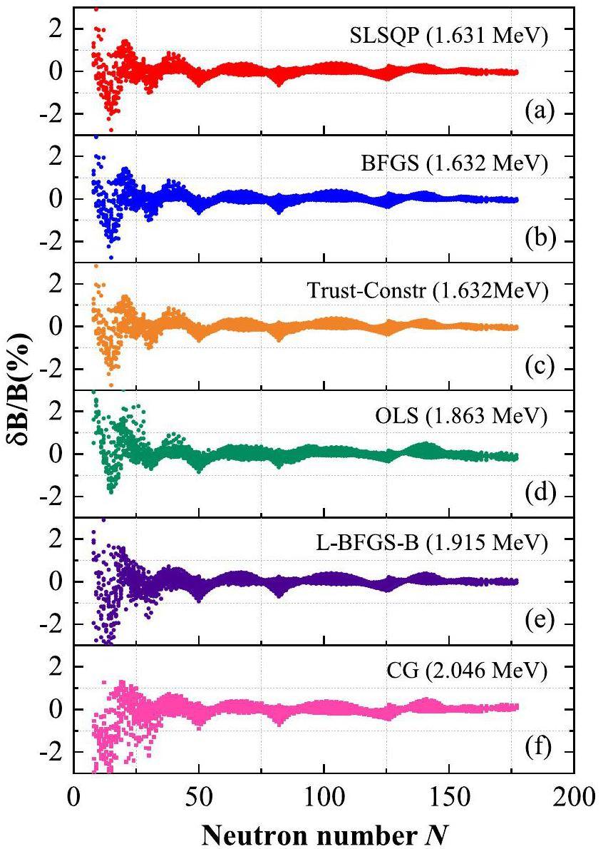
Figure 2 shows the relative error between the theoretical and experimental values of the BW3 mass model obtained by employing the SLSQP and OLS algorithms, where the x-axis represents the neutron number, the y-axis represents the atomic number, and the z-axis corresponds to the relative error percentage
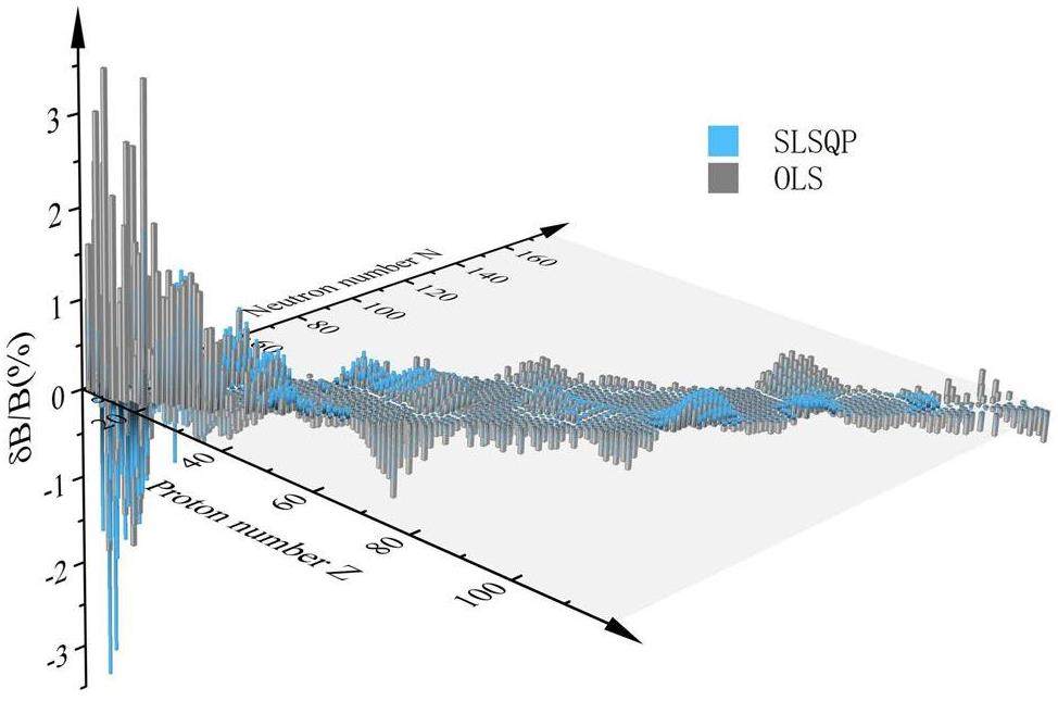
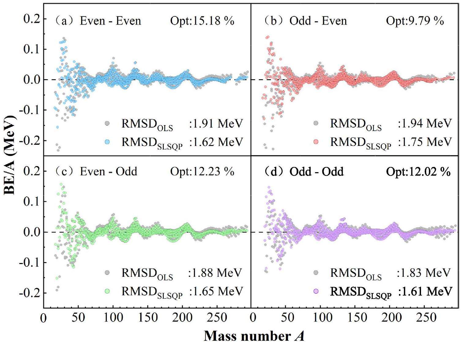
Figure 3 shows the performance of the SLSQP algorithm with regard to even-even, odd-odd, and odd-A nuclei. The optimization effect of the SLSQP algorithm on different types of nuclei exhibit significant differences. The improvement is most pronounced for even-even nuclei, whereas certain optimization results can also be attained for odd-A and odd-odd nuclei. Figure 3a shows that for even-even nuclei [48] (both Z and N are even), the SLSQP algorithm provides a significant reduction in RMSD [28] by 0.29 MeV, with a performance improvement of approximately 15.18%, achieving a more substantial optimization in the entire nuclei region compared with the theoretical value of the BW3 model with OLS coefficients. In Fig. 3b, for odd-Z and even-N nuclei, after the SLSQP optimization, the model RMSD is reduced by 0.19 MeV, with a performance improvement of approximately 9.79%. Similarly, in Fig. 3c, for even-Z and odd-N nuclei, the model RMSD is reduced by 0.23 MeV, with a performance improvement of approximately 12.23%. Notably, in the medium-nuclei region, the optimization results are closer to the experimental values. For odd-odd nuclei (both Z and N are odd), Fig. 3d shows that after SLSQP optimization, the model RMSD is reduced by 0.22 MeV and the performance is improved by approximately 12.02%. In particular, in the heavy-nuclei region, the optimization results are closer to the experimental values. These results further validate the effectiveness of the SLSQP algorithm for mass model optimization.
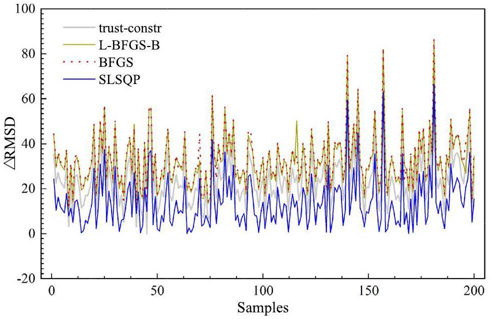
To test the generality of the SLSQP method, we devised 200 sample mass formulae by randomly selecting parameters from the F-parameters in the δE term of the Eisospin mass model. As mentioned previously, the Eisospin mass model consists of two parts: the ELDM term, which contains nine M-parameters derived from the liquid drop model, and the δE term, which encompasses more than 100 F-parameters. If we set M = 4 in the Eisospin mass model, then 144 F-parameters are obtained. Subsequently, we compared the results with the nuclear mass dataset AME2020 and found that the RMSD was 1.268 MeV in this situation. Next, we tested the contributions of these F-parameters individually and identified 53 parameters that had obvious effects on the binding energy. Subsequently, we randomly selected 10 F-parameters from the 53 F-parameters and combined them with nine M-parameters to form a sample mass formula. Thus, we devised 200 sample mass formulas to test the proposed algorithms presented in this work. The SLSQP method outperformed the other algorithms in terms of both error and convergence speed.
As shown in Fig. 4, the SLSQP algorithm performs significantly better than the BFGS and L-BFGS-B algorithms. For example, at the 48th sample point, the
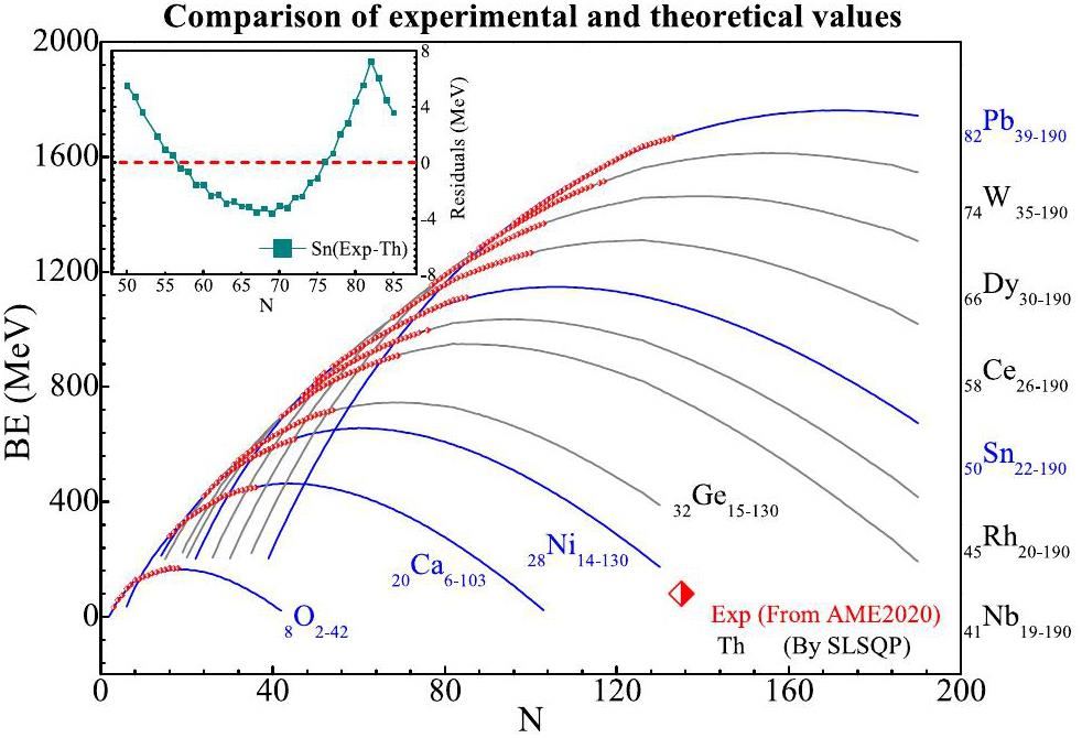
To verify the effectiveness of the SLSQP algorithm, the experimental and theoretical values were compared, as illustrated in Fig. 5. The experimental binding energy values were obtained from AME2020, whereas the theoretical values were obtained by optimizing the BW3 mass model using the SLSQP method. Among the experimental values, the maximum binding energy for the O isotopes is currently measured at 24O16, with a binding energy value of 168.95 MeV. Beyond this isotope, the binding energy decreases as N increases. The SLSQP-optimized theoretical model predicts the maximum point to be at 26O18 with a binding energy value of 168.95 MeV, followed by a similar decline in the binding energy with an increase in N. For the other isotope chains, the experimental binding energy values exhibit an overall increasing trend without reaching a maximum. By optimizing the BW3 nuclear mass model using the SLSQP method, the following maximum binding energy points are predicted for these isotope chains: 64Ca=464.33 MeV, 88Ni=656.72 MeV, 123Nb=950.29 MeV, 141Rh=1035.66 MeV, 100Ge=745.77 MeV, 156Sn=1148.31 MeV, 184Ce=1311.84 MeV, 206Dy=1463.63 MeV, 230W=1613.36 MeV, 252Pb=1761.89 MeV.
Conclusions
In this study, we investigated an improved mass model with a higher-order symmetry energy term by employing several algorithms. The SLSQP algorithm demonstrated the best performance in terms of both root mean square errors and computational efficiency. This algorithm reduced the global RMSD from 1.863 MeV to 1.631 MeV (12.45% reduction). The odd (even) numbers of protons and neutrons are discussed, and the SLSQP algorithm reduced the local RMSD from 1.91 MeV to 1.62 MeV (15.18% optimization) when the nuclei have even numbers of both protons and neutrons. The local RMSD is reduced from 1.83 MeV to 1.61 MeV when the nuclei have odd numbers of protons and neutrons. With an odd (even) number of protons (neutrons), the local RMSD decreases from 1.94 MeV to 1.75 MeV (9.79% optimization). The local RMSD is reduced from 1.88 MeV to 1.65 MeV (12.23% optimization) when the number of protons is even and the number of neutron is odd. We tested these algorithms using 200 sample mass formulas derived from the Eisospin mass model. Each sample mass formula includes 19 free parameters, of which nine are M-parameters derived from the liquid drop model and 10 are F-parameters from the δE term of the Eisospin mass model. The SLSQP method provides better performance than the other algorithms in terms of errors and convergence speed. According to this study, the SLSQP algorithm is suitable for handling large-scale multiparameter optimization tasks in nuclear physics.
Self-consistent mean-field models for nuclear structure
. Rev. Mod. Phys 75, 121-180 (2003). https://doi.org/10.1103/RevModPhys.75.121Recent trends in the determination of nuclear masses
. Rev. Mod. Phys 75, 1021-1082 (2003). https://doi.org/10.1103/RevModPhys.75.1021Novel Techniques for Constraining Neutron-Capture Rates Relevant for r -Process Heavy-Element Nucleosynthesis
. Prog. Part. Nucl. Phys 107, 69-108 (2019). https://doi.org/10.1016/j.ppnp.2019.04.002Masses of exotic nuclei
. Prog. Part. Nucl. Phys 120,The limits of the nuclear landscape
. Nature 486, 509-512 (2012). https://doi.org/10.1038/nature11188The AME 2020 atomic mass evaluation (I). Evaluation of input data, and adjustment procedures
. Chinese Phys. C 45,The AME 2020 atomic mass evaluation (II). Tables, graphs and references
. Chinese Phys. C 45,Nuclear ground-state masses and deformations: FRDM(2012)
. At. Data Nucl. Data Tables 109–110, 1-204 (2016). https://doi.org/10.1016/j.adt.2015.10.002Zur Theorie der Kernmassen
. Z. Physik 96, 431-458 (1935). https://doi.org/10.1007/BF01337700Nuclear Physics A
. Stationary States of Nuclei. Rev. Mod. Phys 8, 82 (1936). https://doi.org/10.1103/RevModPhys.8.82Better insight into the Strutinsky method
. Phys. Rev. C 100,Bethe-Weizsacker semiempirical mass formula coefficients 2019 update based on AME2016
. Nucl. Sci. Tech 31, 9 (2020). https://doi.org/10.1007/s41365-019-0718-8Accuracy versus predictive power in nuclear mass tabulations
. Phys. Rev. C 106,New Finite-Range Droplet Mass Model and Equation-of-State Parameters
. Phys. Rev. Lett 108,Nuclidic Mass Formula on a Spherical Basis with an Improved Even-Odd Term
. Prog. Theor. Phys 113, 305 (2005). https://doi.org/10.1143/PTP.113.305Optimal shapes and fission barriers of nuclei within the liquid drop model
. Phys. Rev. C 79,Further explorations of Skyrme-Hartree-Fock-Bogoliubov mass formulas. XII. Stiffness and stability of neutron-star matter
. Phys. Rev. C 82,Further explorations of Skyrme-Hartree-Fock-Bogoliubov mass formulas. XIII. The 2012 atomic mass evaluation and the symmetry coefficient
. Phys. Rev. C 88,Mean free path in the relativistic mean field
. Phys. Rev. C 44, 1944 (1991). https://doi.org/10.1103/PhysRevC.44.1944Precise effective masses from density functional perturbation theory
. Phys. Rev. B 93,Mutual influence of terms in a semi-empirical mass formula
. Nucl. Phys. A. 798, 29-60 (2008). https://doi.org/10.1016/j.nuclphysa.2007.10.011Nuclear masses and deformations
. Nucl. Phys 81, 1-60 (1966). https://doi.org/10.1016/S0029-5582(66)80001-9Temperature dependence of the symmetry energy and neutron skins in Ni, Sn, and Pb isotopic chains
. Phys. Rev. C 95,Application of a Coulomb energy density functional for atomic nuclei: Case studies of local density approximation and generalized gradient approximation
. Phys. Rev. C 97,Surface and curvature properties of charged strangelets in compact objects
. Phys. Rev. C 103,On the Consequences of the Symmetry of the Nuclear Hamiltonian on the Spectroscopy of Nuclei
. Phys. Rev 51, 106 (1937). https://doi.org/10.1103/PhysRev.51.106Nuclear Structure from a Simple Perspective
. Oxford. Acad 32, 358-358 (2001). https://doi.org/10.1093/acprof:oso/9780198507246.001.0001Coefficients and terms of the liquid drop model and mass formula
. Phys. Rev. C 73,Nuclear mass predictions based on Bayesian neural network approach with pairing and shell effects
. Phys. Lett. B 778, 48-53 (2018). https://doi.org/10.1016/j.physletb.2018.01.002Random forest-based prediction of decay modes and half-lives of superheavy nuclei
. Nucl. Sci. Tech 34, 204 (2023). https://doi.org/10.1007/s41365-023-01354-5Predictions of nuclear charge radii based on the convolutional neural network
. Nucl. Sci. Tech 34, 152 (2023). https://doi.org/10.1007/s41365-023-01308-xPrediction of nuclear charge density distribution with feedback neural network
. Nucl. Sci. Tech 33, 153 (2022). https://doi.org/10.1007/s41365-022-01140-9Multiple constraints on nuclear mass formulas for reliable extrapolations
. Phys. Rev. C 107,Set of Nuclear-Mass Relations and a Resultant Mass Table
. Rev. Mod. Phys 41, S1-S80 (1969). https://doi.org/10.1103/RevModPhys.41.S1Simple nuclear mass formula
. Phys. Rev. C 90,An experimental study on local and global optima of linear antenna array synthesis by using the sequential least squares programming
. Appl. Soft. Comput. 148,Improved nuclear mass formula with an additional term from the Fermi gas model
. Nucl. Sci. Tech 35, 91 (2024). https://doi.org/10.1007/s41365-024-01450-0Nuclear pairing models
. Nucl. Phys. A 536, 20-60 (1992). https://doi.org/10.1016/0375-9474(92)90244-EOrdinary least squares estimation of parameters of linear model
. J. Math. Comput. Sci. 11, 2015-2030 (2021). https://doi.org/10.28919/jmcs/5454Robust approximation of chance constrained optimization with polynomial perturbation
. Comput. Optim. Appl. 89, 977-1003 (2024). https://doi.org/10.1007/s10589-024-00602-7LSLOpt: An open-source implementation of the step-length controlled LSL-BFGS algorithm
. J. Comput. Chem. 42, 1095-1100 (2021). https://doi.org/10.1002/jcc.26522A Class New Hybrid Conjugate Gradient Method for Unconstrained Optimization
. J. Comput. Chem. 12, 1941-1949 (2015). https://api.semanticscholar.org/CorpusID:124611131On the Global Convergence of a Projective Trust Region Algorithm for Nonlinear Equality Constrained Optimization
. Acta. Math. Sin.-English Ser. 34, 1804-1828 (2018). https://doi.org/10.1007/s10114-018-7063-4The Hessian matrix of Lagrange function
. Linear. Algebra. Appl. 531, 537-546 (2017). https://doi.org/10.1016/j.laa.2017.06.012Interval linear fractional programming: optimal value range of the objective function
. Comp. Appl. Math 39, 261 (2020). https://doi.org/10.1007/s40314-020-01308-2An efficient and robust Lagrange multiplier approach with a penalty term for phase-field models
. J. Comput. Phys 488,Boundedness of the inverse of a regularized Jacobian matrix in constrained optimization and applications
. Optim. Lett 16, 2359-2371 (2022). https://doi.org/10.1007/s11590-021-01829-7Improved radial basis function approach with odd-even corrections
. Phys. Rev. C 94,The authors declare that they have no competing interests.


