Introduction
Since the direct discovery of neutrinos by Cowan and Reines at the Savannah River reactor power plant in 1956 [1], reactor neutrino experiments have played a pivotal role in the advancement of neutrino physics. Reactor neutrinos are also known as reactor antineutrinos because they are composed exclusively of electron antineutrinos (
Fissile isotope antineutrino spectra and fluxes have been evaluated several times in the past decades. The methodologies employed can be classified into three major categories comprising summation [10], conversion [11, 12], and extraction methods [13-15]. The summation method, i.e., the ab initio approach, utilizes information on fission products and decays from nuclear databases to calculate and sum the contributions of all possible beta decay chains to
The current general practice in experiments for extracting fissile isotope antineutrino spectra involves first unfolding the reconstructed prompt energy spectrum to obtain an antineutrino energy spectrum weighted by the IBD cross section, and then further fitting the unfolded spectrum with the χ2 minimization method to extract individual or combined isotope antineutrino spectra [14, 15, 26, 27]. Unfolding is a common technique used in high-energy physics (HEP) to disentangle detector effects, correct migration effects, suppress fluctuations, and reconstruct approximate distributions of quantities. Common methods for unfolding include singular value decomposition (SVD) [29], Wiener SVD [30], and Bayesian iterations [31]. In the Daya Bay experiment, these methods were used to yield consistent extraction results. Although the Wiener-SVD method produces the smallest unfolded spectrum mean square error (MSE) within the energy range of 3-6 MeV, it does not perform as well as the other methods outside this energy range because of the large statistical fluctuations in the intrinsic neutrino energy spectrum [14]. To obtain more precise solutions, the number of bins for the unfolded spectrum in experiments is typically limited to that of the intrinsic spectrum [32]. Although this simplifies the subsequent fitting process for extracting the specific fission isotope antineutrino spectrum, it also suppresses the fine structure of the spectrum shape.
In our previous study [33], we proposed a machine learning method in which a convolutional neural network (CNN) model is employed to extract fission isotope antineutrino spectra from the unfolded prompt energy spectrum in a virtual short-baseline reactor neutrino experiment. The analysis results demonstrate that the proposed CNN model can achieve subpercentage uncertainties in the extracted 235U and 239Pu antineutrino spectra whereas the 238U and 241Pu antineutrino spectra need to be constrained via prior knowledge during the fitting process. In this study, we extend the method and establish a feedforward neural network (FNN) model to resolve this extraction problem. This new method is designed to directly extract the antineutrino spectra of the four fission isotopes from the reconstructed prompt energy spectrum without highlighting the unfolding process or any constraints on the spectra while better preserving the fine structure of the extracted spectra.
The remainder of this paper is organized as follows: In Sect. 2, we present the antineutrino spectra of the IBD reactions and the generation of the simulation dataset for this study. In Sect. 3, we introduce the conceptual and technical details of the proposed FNN model and its training strategies. In Sect. 4, we compare the performance of this new method in extracting fission isotope antineutrino spectra with that of the benchmark traditional method, that is, the χ2 minimization method, and discuss the obtained results. Finally, a summary and future outlook are presented in Sect. 5.
Dataset generation for FNN model
In this study, we constructed a virtual reactor neutrino experiment in a layout comprising a PWR and a detector. To verify the feasibility of the virtual experiment, we referred to the Daya Bay [14] and Taishan Antineutrino Observatory (TAO, also known as JUNO-TAO) [34, 35] experiments, and made the following assumptions about the experimental parameters: The reactor is operated for 1800 days at a full thermal power of 2.9
IBD yield prediction
The Huber-Mueller model is a theoretical framework for predicting the antineutrino spectra produced by the fission reactions of four isotopes in reactors. Each of these isotopic antineutrino spectrum can be parameterized using the exponent of a fifth-order polynomial as follows:
The antineutrino yield per fission can be expressed as
In the standard three-flavor neutrino oscillation framework, the survival probability Pee of
For short-baseline reactor neutrino experiments, considering that the term involving Δ21 is negligible and
As the
To simplify the calculation, we assumed that the detector has no energy leakage or LS nonlinearity [32]. Thus, the prompt energy
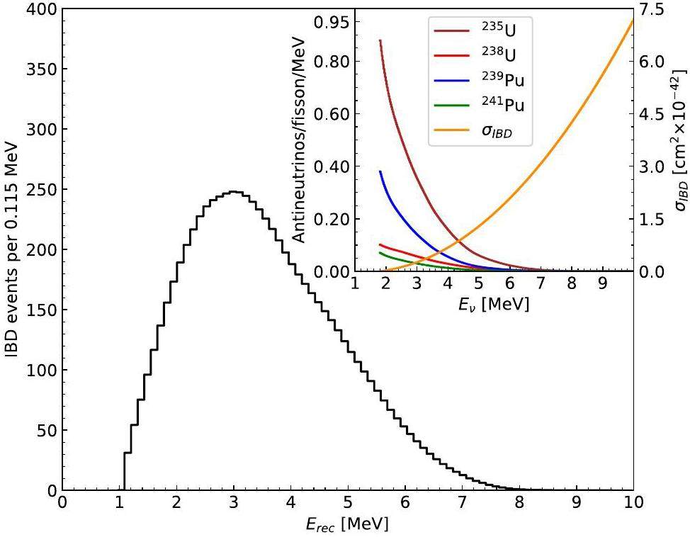
For simplicity, we set p0 = 0.08, p1 = 0, and p2 = 0 in this study for an energy resolution of 8% at 1 MeV in the detector. Therefore, under full reactor power and classical fission fractions conditions [32], the detector observes the energy spectrum of the IBD events (i.e., the reconstructed prompt energy spectrum) distorted by the RAA in one day, as shown in Fig. 1, and approximately 7473 IBD events are recorded.
Simulated samples and targets in dataset
Considering the significant computational resources and time required for the integral terms in Eq. (8), Eq. (8) is typically converted to a discrete summation or matrix multiplication equivalent form in practical computations. In this study, the integral form of the reconstructed prompt energy spectrum is rewritten as an element of the row matrix
Each row of
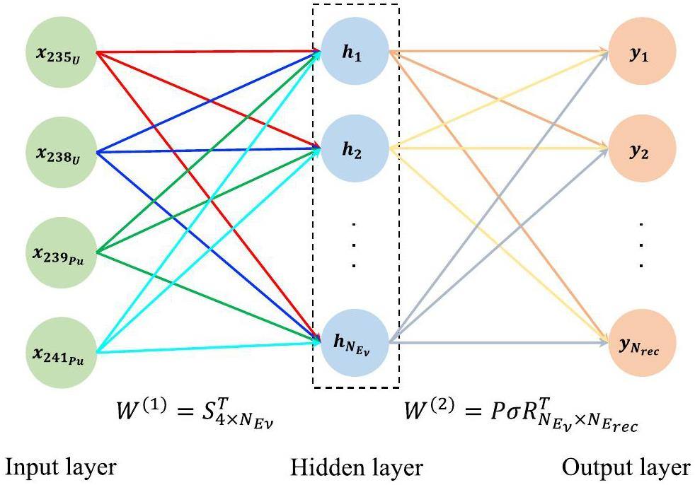
The matrix multiplication relation in Eq. (11) provides the mathematical foundation for constructing the FNN architecture presented in Sect. 3. Furthermore, X1×4 and
As described in Eq. (12), the fission fraction varies dynamically with burn-up as the reactor operates. In each reactor core refueling cycle, the cycle burn-up can be calculated as [32]
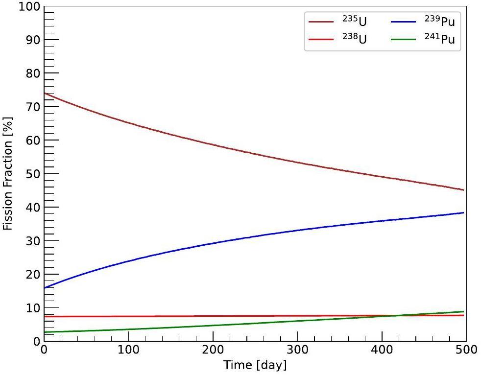
Under the assumption that the thermal power and fissile fractions for the four main isotopes of the reactor are constant within each day, we accumulated the exposure over each 3-day interval as a sample to create a dataset of 600 simulated samples and their corresponding targets for subsequent analysis.
Implementation of FNN model
Machine learning algorithms such as neural network (NN) models have attracted increasing attention from high-energy and nuclear physics researchers [33, 40-44]. However, most of these applications are characterized by black-box models in which the meaning of the model parameters are challenging to understand or interpret. In this section, we present a FNN-based white-box model where each layer and parameter has a clear physical or mathematical meaning, thereby ensuring the interpretability of the model.
Mathematical foundations of FNN model
The NN is a powerful machine learning model that has been widely explored and applied across various fields. The universal approximation theorem [45, 46] implies that any continuous function can be approximated with arbitrary precision using an appropriate NN, even if the NN is an FNN with only one hidden layer containing a sufficient number of neurons. However, the internal structure and parameters of the NN in such scenarios often lack physical meaning or interpretability. This results in black-box models, which are not fully trusted by high-energy physicists. Therefore, we designed and implemented a white-box NN model in this study for converting the mathematical mapping function in Eq. (11) to a FNN model.
An FNN is typically composed of one to several single-layer perceptrons, which are considered the fundamental building units of the FNN and play a vital role in its overall functionality [47]. Each perceptron in the FNN follows the computational flow shown in Fig. 3 to process data. Forward and backward propagation are two phases in the NN training process that interact to optimize network performance.
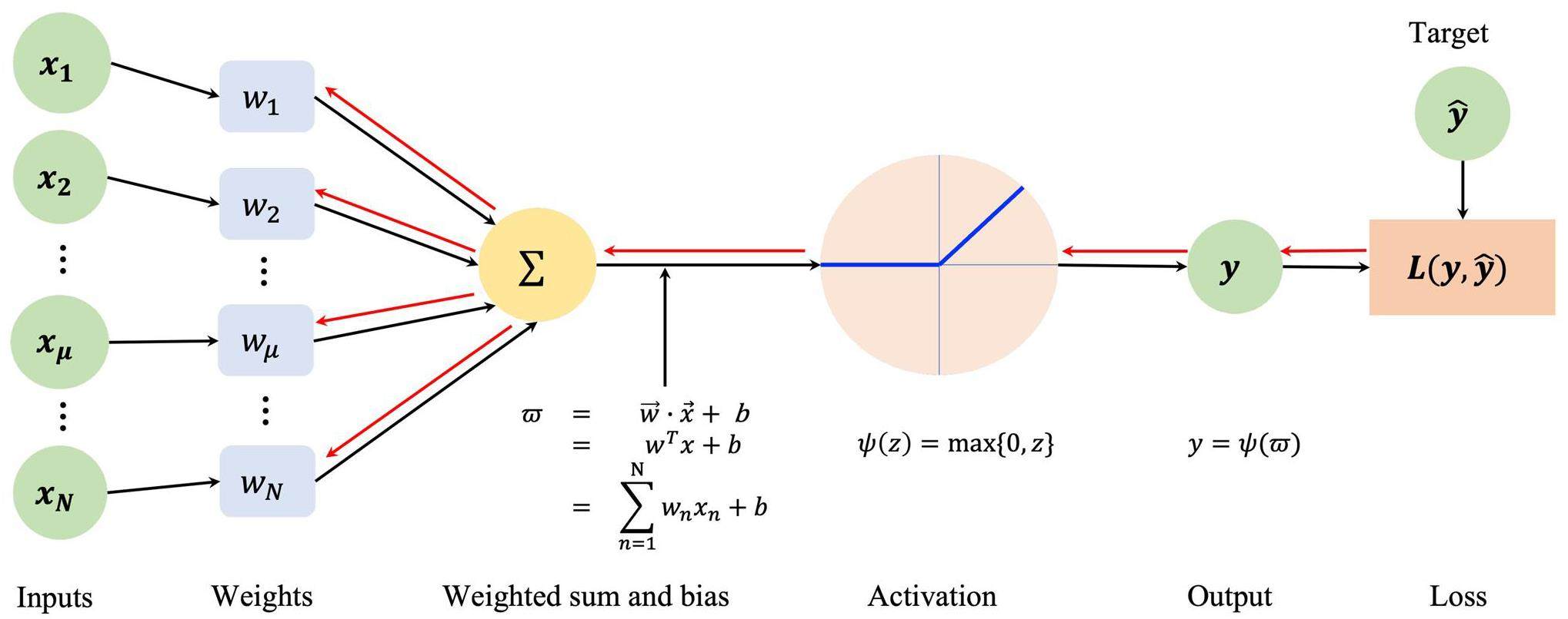
During the forward propagation phase, the perceptron performs computation by computing the dot product of the input vector
To allow matrix multiplication in the perceptrons, the bias b must be eliminated, i.e., set to zero. The absence of negative values in our data flow justifies the use of the default rectified linear unit (ReLU) activation function, which is defined as
As shown in Fig. 4, the architecture of the FNN model consists of three layers comprising, from left to right, the input, hidden, and output layers with four,
Training strategy
All the samples generated in Sect. 2.2 were utilized solely to train the FNN model. The validation and testing processes were omitted. This approach was chosen because our aim is to minimize the loss function during the training process to determine the optimal W(1) for extracting the four main isotopic antineutrino spectra. Our focus is on optimizing spectra extraction performance rather than evaluating model performance across various datasets, as well as on simplifying the process and aligning with our primary research objective.
The loss function is a fundamental component in deep-learning models. It serves as the criterion for evaluating how well the model predictions match the actual outcomes and provides a numerical indicator of model accuracy. The Combined Neyman-Pearson (CNP) chi-square model is a statistical model frequently employed in HEP experiments to quantify the error between predicted and measured values [48]. Based on this model, we define the loss function for the FNN model as
After defining the loss function, it is essential to select a suitable optimizer, learning rate schedule, batch size, and epoch, among other hyperparameters. Following hyperparameter tuning using the Optuna framework [49] and extensive testing, we developed two training strategies denoted as the short- and long-epoch strategies to investigate the performance of the FNN model in extracting the antineutrino spectra of the four fission isotopes from the reconstructed prompt energy spectrum [50]. As shown in Table 1, a critical commonality between these two strategies is the segmentation of the hidden layer in the FNN model into multiple partitions or parallel hidden layers. This setup allows distinct learning and weight decay rates to be assigned to each partition to facilitate differential performance outcomes. Because the focus in this study is not on the isotope antineutrino spectra above 8 MeV, i.e., in the (303, 401] partition or the matrix
| Strategy | Short-epoch | Long-epoch |
|---|---|---|
| Epoch | 2×10⁶ | 2×10⁶ |
| Optimizer | AdamW | Adam |
| Hidden layer partitions | [1], (1, 180], (180, 225], (225, 303], (303, 401] | |
| Learning rates for hidden layer | [3.4892×10⁻⁴, 9.9485×10⁻⁴, 2.754×10⁻⁴, 1.8272×10⁻⁴, 0] | |
| Weight decay rates for hidden layer | [7.418×10⁻³, 7.748×10⁻³, 4.155×10⁻³, 9.999×10⁻³, 0] | [0, 0, 0, 0, 0] |
| Learning rate for output layer | 0 | |
| Weight decay for output layer | 0 | |
| Learning rate scheduler | ReduceLROnPlateau (factor=0.32, patience=1×10²) | ReduceLROnPlateau (factor=0.32, patience=1×10⁴) & epoch≥2×10⁵ |
| Batch size | 30 |
As indicated by their names, the main distinction between the short- and long-epoch strategies lies in the epochs. The short-epoch strategy leverages the AdamW [51] optimizer with non-zero weight decay rates for faster loss reduction. In contrast, in the long-epoch strategy, the Adam [52] optimizer is applied without weight decay, i.e., the weight decay rates are set to zero. Superior convergence results were obtained using the long-epoch strategy. The results are presented and discussed in Sect. 4. As illustrated in Table 1, these circumstances also led to minor differences in the configurations of the learning rate schedulers. Nonetheless, the same metric, i.e., the sum of the losses for all samples denoted as
We also extracted the antineutrino spectra of the four fission isotopes using the χ2 minimization method to provide a comparison and benchmark for the FNN model. We employed the Minuit2 minimization library from ROOT [53] to implement this method.
The FNN model was implemented using PyTorch [54], a Python-based deep learning library that supports both CPU and GPU platforms and is one of the mainstream tools for developing and training NN models. A NVIDIA GeForce RTX 3060 Ti GPU platform was used to deploy the FNN model, whereas tasks involving Optuna and ROOT were performed on two identical servers, each of which was equipped with two 28-core Intel(R) Xeon(R) Gold 6330 CPUs @ 2.00 GHz.
Results and discussions
To facilitate the discussion and comparative analysis of the short- and long-epoch strategies of our FNN model and the χ2 minimization method, we first consider their performance in fitting all the samples and reducing the losses. As shown in Fig. 5, did the loss
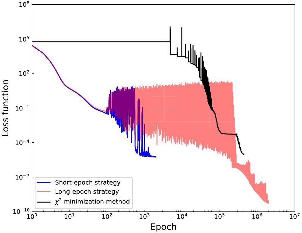
The short-epoch strategy can rapidly reduce the loss in the early stages of training mainly because of the regularization effects and optimization efficiency due to the combination of nonzero weight decay rates and the AdamW optimizer. However, in the later stages of training, the model must be able to respond to small changes in the loss function for fine adjustments of the parameters. Weight decay may interfere with this process and make it challenging for the model to determine the optimal solution within regions of small loss function gradients.
Figure 6 shows a comparison of the performance in extracting the antineutrino spectra of the four isotopes using these three approaches. The extraction performance decreases in the order of the long-epoch strategy, short-epoch strategy, and χ2 minimization method. The FNN model accurately extracted the antineutrino spectra of 235U, 239Pu, and 241Pu in the energy range of 2-5 MeV. The FNN model with the short-epoch strategy achieved relative errors of less than 2% in the 5-8 MeV range, which decreased to less than 1% with the long-epoch strategy. In comparison, the χ2 minimization method achieved relative extraction errors of less than 2% and 3% for these three isotopes in the respective energy ranges. For the isotope 238U, both the short-epoch strategy and χ2 minimization method showed relatively poor extraction performance compared to that for the other isotopes. The maximum extraction relative errors in the 2-8 MeV range are approximately 4% and 8%, respectively, whereas only the long-epoch strategy maintained relative errors of less than 1%.
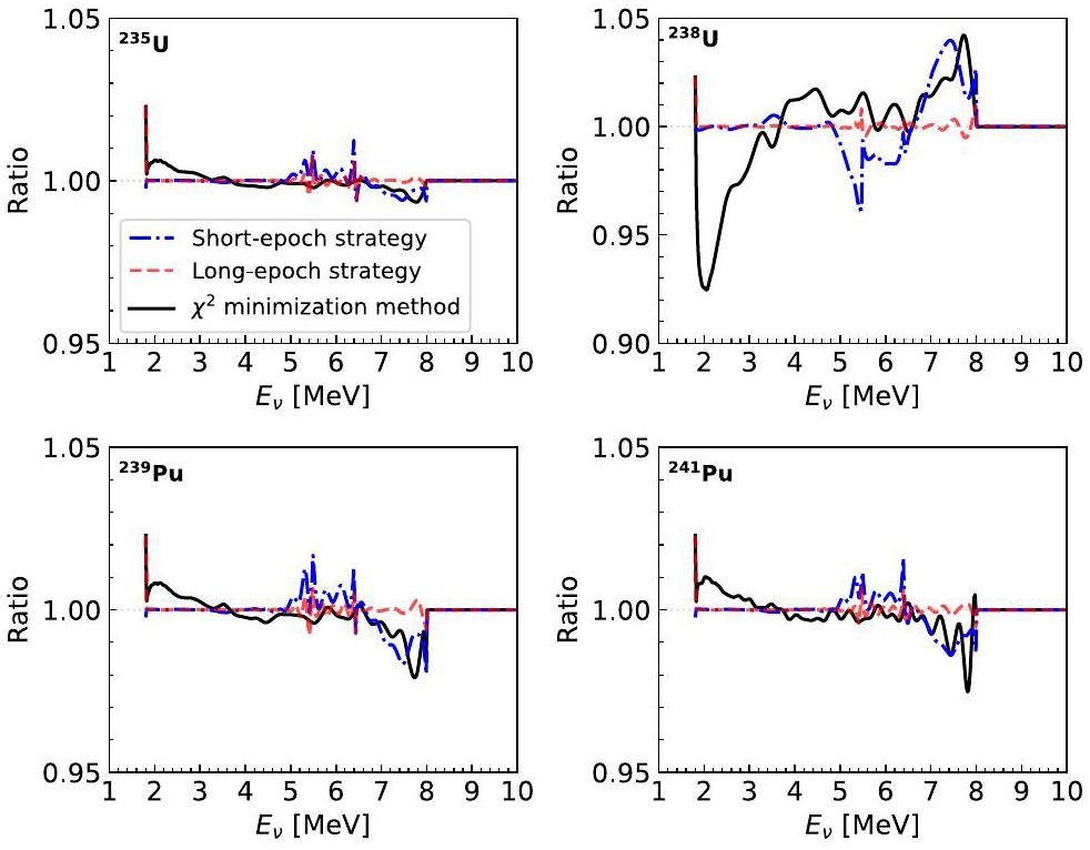
It is worth noting that although 241Pu has a lower average fission fraction throughout the entire refueling cycle compared to 238U, the extraction performance for the former is better in all the extraction approaches. This indicates that in addition to large fission fractions, significant variations are also crucial for extracting isotopic antineutrino spectra accurately. Greater variations produce better extraction results. This is further confirmed by the extraction performance for the 235U and 239Pu antineutrino spectra. Therefore, such long epochs are employed in the long-epoch strategy primarily to enhance the extraction performance for 238U. Overall, regardless of the extraction approach used, the extraction performance for the isotopic antineutrino spectra in descending order is as follows: 235U, 239Pu, 241Pu, and 238U.
The above results and discussion reveal that because of the exceptional capability of NNs in optimizing large-scale parameters, the FNN model achieved faster and more effective convergence than the traditional χ2 minimization method. Based on PyTorch’s extensive array of optimization algorithms [55], various model training strategies can be designed to satisfy the practical requirements for extracting isotope antineutrino spectra. Moreover, executing spectrum extraction algorithms on GPU platforms can significantly increase the inference speed of the process, thereby improving extraction efficiency.
Summary and outlook
In this study, we presented an FNN model designed to infer and extract the corresponding antineutrino spectra generated by the fission of 235U, 238U, 239Pu, and 241Pu from the reconstructed prompt energy spectrum measured by the detector in a reactor neutrino experiment. Using a simulated short-baseline reactor neutrino experiment with an exposure of
By comparing the extraction effects of the short- and long-epoch training strategies for our FNN model with the traditional χ2 minimization method, as shown in Fig. 6, we found that the FNN model converged faster and better, and the performance of the three approaches for extracting the isotope antineutrino spectra in descending order is as follows: long-epoch strategy, short-epoch strategy, and χ2 minimization method. Furthermore, the relative extraction errors of the antineutrino spectra for the four isotopes are reduced to less than 1% in the 2-8 MeV range of interest by the FNN model with the long-epoch strategy, which is better than the error of 8% or less obtained using the χ2 minimization method in the control group. These results show that the FNN model has considerable potential for extracting fission isotope antineutrino spectra.
In the near future, TAO will serve as a satellite experiment of JUNO and achieve an energy resolution exceeding 2% at 1 MeV in measuring reactor antineutrinos [34]. Its primary physics goals include constraining the fine structures of isotope antineutrino spectra and providing a model-independent reference spectrum for JUNO and a benchmark measurement to test nuclear databases. Employing the FNN model in high-precision experiments such as TAO would therefore be an excellent match. In addition, depending on the research objectives, new NN models can be developed using the methodologies outlined in this study to further investigate a broader range of physics topics such as unfolding, neutrino oscillation parameter measurements, sterile neutrino searches, and reactor monitoring. For example, the unfolded neutrino energy spectrum is represented by the output of the hidden layers in our FNN model, which can achieve a relative error of less than 1% in the 2-8 MeV range.
Detection of the free antineutrino
. Phys. Rev. 117, 159-173 (1960). https://doi.org/10.1103/PhysRev.117.159Nuclear reactor safeguards and monitoring with anti-neutrino detectors
. J. Appl. Phys. 91, 4672 (2002). https://doi.org/10.1063/1.1452775Antineutrino spectra and their applications. Tech. rep.
,Report of the Topical Group on Neutrino Applications for Snowmass 2021
. in:Neutrino physics with JUNO
. J. Phys. G 43,Sterile neutrino search at the NEOS experiment
. Phys. Rev. Lett. 118,Improved short-baseline neutrino oscillation search and energy spectrum measurement with the PROSPECT experiment at HFIR
. Phys. Rev. D 103,Constraints on elastic neutrino nucleus scattering in the fully coherent regime from the CONUS experiment
. Phys. Rev. Lett. 126,Reactor neutrino liquid xenon coherent elastic scattering experiment
. Phys. Rev. D 110,New antineutrino energy spectra predictions from the summation of beta decay branches of the fission products
. Phys. Rev. Lett. 109,Absolute measurement of the beta spectrum from 235U fission as a basis for reactor antineutrino experiments
. Phys. Lett. B 99, 251-256 (1981). https://doi.org/10.1016/0370-2693(81)91120-5The reactor antineutrino anomaly
. Phys. Rev. D 83,Extraction of the 235U and 239Pu antineutrino spectra at Daya Bay
. Phys. Rev. Lett. 123,Antineutrino energy spectrum unfolding based on the Daya Bay measurement and its applications
. Chin. Phys. C 45,Joint determination of reactor antineutrino spectra from 235U and 239Pu fission by Daya Bay and PROSPECT
. Phys. Rev. Lett. 128,Improved predictions of reactor antineutrino spectra
. Phys. Rev. C 83,Experimental beta-spectra from 239Pu and 235U thermal neutron fission products and their correlated antineutrino spectra
. Phys. Lett. B 118, 162-166 (1982). https://doi.org/10.1016/0370-2693(82)90622-0Determination of the antineutrino spectrum from 235U thermal neutron fission products up to 9.5 MeV
. Phys. Lett. B 160, 325-330 (1985). https://doi.org/10.1016/0370-2693(85)91337-1Anti-neutrino Spectra From 241Pu and 239Pu thermal neutron fission products
. Phys. Lett. B 218, 365-368 (1989). https://doi.org/10.1016/0370-2693(89)91598-0Experimental determination of the antineutrino spectrum of the fission products of 238U
. Phys. Rev. Lett. 112,Determination of antineutrino spectra from nuclear reactors
. Phys. Rev. C 84,Double chooz θ13 measurement via total neutron capture detection
. Nature Phys. 16, 558-564 (2020). https://doi.org/10.1038/s41567-020-0831-yMeasurement of reactor antineutrino oscillation amplitude and frequency at RENO
. Phys. Rev. Lett. 121,New results from RENO and the 5 MeV excess
. AIP Conf. Proc. 1666,NEOS data and the origin of the 5 MeV bump in the reactor antineutrino spectrum
. Phys. Rev. Lett. 118,Final measurement of the 235U antineutrino energy spectrum with the PROSPECT-I detector at HFIR
. Phys. Rev. Lett. 131,Joint measurement of the 235U antineutrino spectrum by PROSPECT and STEREO
. Phys. Rev. Lett. 128,STEREO neutrino spectrum of 235U fission rejects sterile neutrino hypothesis
, Nature 613, 257-261 (2023). https://doi.org/10.1038/s41586-022-05568-2SVD approach to data unfolding
. Nucl. Instrum. Meth. A 372, 469-481 (1996). https://doi.org/10.1016/0168-9002(95)01478-0Data unfolding with Wiener-SVD method
. JINST 12,A Multidimensional unfolding method based on Bayes’ theorem
, Nucl. Instrum. Meth. A 362, 487-498 (1995). https://doi.org/10.1016/0168-9002(95)00274-XImproved measurement of the reactor antineutrino flux and spectrum at Daya Bay
. Chin. Phys. C 41,Decomposition of fissile isotope antineutrino spectra using convolutional neural network
. Nucl. Sci. Tech. 34, 79 (2023). https://doi.org/10.1007/s41365-023-01229-9TAO conceptual design report: A precision measurement of the reactor antineutrino spectrum with sub-percent energy resolution
. https://doi.org/10.48550/arXiv.2005.08745Design optimization of juno-tao plastic scintillator with wls-fiber and sipm readout
. Nucl. Sci. Tech. 34, 99 (2023). https://doi.org/10.1007/s41365-023-01175-6Improved calculation of the energy release in neutron-induced fission
. Phys. Rev. C 88,Review of particle physics
. PTEP 2022Calibration strategy of the JUNO experiment
. JHEP 03, 004 (2021). https://doi.org/10.1007/JHEP03(2021)004Precise quasielastic neutrino/nucleon cross-section
. Phys. Lett. B 564, 42-54 (2003). https://doi.org/10.1016/S0370-2693(03)00616-6Improvement of machine learning-based vertex reconstruction for large liquid scintillator detectors with multiple types of PMTs
. Nucl. Sci. Tech. 33, 93 (2022). https://doi.org/10.1007/s41365-022-01078-yVertex and energy reconstruction in JUNO with machine learning methods
. Nucl. Instrum. Meth. A 1010,Prediction of nuclear charge density distribution with feedback neural network
. Nucl. Sci. Tech. 33, 153 (2022). https://doi.org/10.1007/s41365-022-01140-9High-energy nuclear physics meets machine learning
. Nucl. Sci. Tech. 34, 88 (2023). https://doi.org/10.1007/s41365-023-01233-zNuclear mass based on the multi-task learning neural network method
. Nucl. Sci. Tech. 33, 48 (2022). https://doi.org/10.1007/s41365-022-01031-zApproximation by superpositions of a sigmoidal function
. Math. Control Signals Syst. 2, 303-314 (1989). https://doi.org/10.1007/BF02551274Approximation capabilities of multilayer feedforward networks
. Neural Networks 4, 251-257 (1991). https://doi.org/10.1016/0893-6080(91)90009-tCombined Neyman–Pearson chi-square: An improved approximation to the Poisson-likelihood chi-square
. Nucl. Instrum. Meth. A 961,Optuna: A next-generation hyperparameter optimization framework
. in:ReduceLROnPlateau class
. https://pytorch.org/docs/stable/generated/torch.optim.lr_scheduler.ReduceLROnPlateau.html AccessedDecoupled weight decay regularization
, in:Adam: A method for stochastic optimization
. 2014. https://doi.org/10.48550/arXiv.1412.6980ROOT: An object oriented data analysis framework
. Nucl. Instrum. Meth. A 389, 81-86 (1997). https://doi.org/10.1016/S0168-9002(97)00048-XPyTorch: An imperative style, high-performance deep learning library
. https://doi.org/10.48550/arXiv.1912.01703pytorch_optimizer: optimizer & lr scheduler & loss function collections in PyTorch
. https://github.com/kozistr/pytorch_optimizerAccessedThe authors declare that they have no competing interests.


