Material

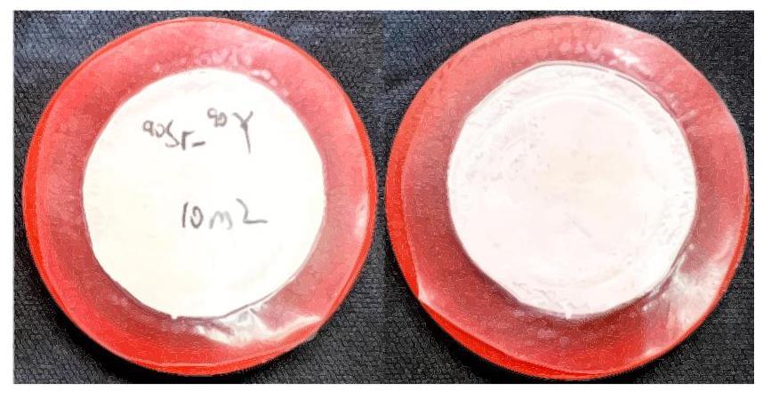
Figure 1 shows ⁹⁰Sr/⁹⁰Y sample source used in the activity error analysis, which was prepared by the Guangdong Radiation Environment Monitoring Technology Center. The method for preparing ⁹⁰Sr/⁹⁰Y sample source was as follows: 10 mL of ⁹⁰Sr/⁹⁰Y standard equilibrium solution with a reference activity of 37.157 Bq/mL was used. Subsequently, strontium [16] and yttrium [17] carriers were added, and oxalic acid was added to precipitate strontium oxalate and yttrium oxalate. The resulting ⁹⁰Sr/⁹⁰Y sample source had a 100% recovery rate. The β sample source had an initial activity of 371.44 Bq and was used for the activity error analysis experiments.

Fig. 1Full-screen View

(color online) Sample source for ⁹⁰Sr/⁹⁰Y

β-Logarithmic Energy Spectrum System

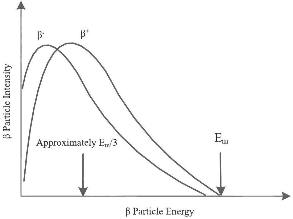
In contrast to the shapes of α and γ decay spectra [18], the β decay spectrum is continuously distributed. Figure 2 shows the β-linear energy spectrum [19]. Given that βnuclides emit βparticles with a continuously distributed energy range from zero to the maximum energy E_m, some βmeasurement systems use a logarithmic processing function to handle the βenergy spectra. Figure 3 illustrates this logarithmic conversion process.

Fig. 2Full-screen View

　β-particle energy spectrum

Fig. 3Full-screen View

(color online) Conversion of β-linear and logarithmic energy spectra

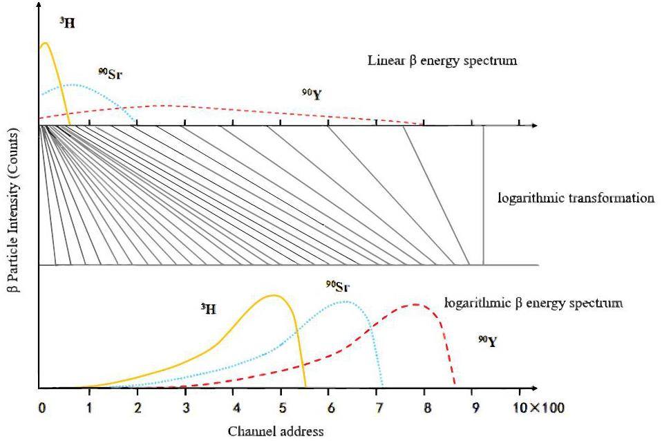
β-Logarithmic energy spectroscopy offers several advantages over linear energy spectroscopy. First, it can significantly enhance the energy resolution in the low-energy range without significantly reducing that in the high-energy range. This solves the problems of inaccuracy and incompleteness of the linear energy spectrum at the low-energy end of the measurement. When analyzing low-activity decay events, the statistical error for each energy channel remains almost constant across the entire energy range of the measurement, owing to the flat background spectral line of the β-logarithmic energy spectrum. Therefore, liquid scintillation spectrometry [20] logarithmic processing of βenergy spectrum is more suitable for conducting energy-spectral analyses of two or more βnuclides.

Fourier Series Function Fitting Model

Curve fitting [21] is a widely used technique in data analysis, statistics, and computer vision, among other fields. Its primary objective is to gain a better understanding of the data, make predictions, and infer the underlying laws by constructing mathematical expressions that match data trends. Common curve-fitting methods include the least-squares, kernel, and spline methods [22, 23].

Least squares [24] is a widely adopted curve-fitting technique. The core concept involves minimizing the sum of the squares of the residuals between the model predictions and actual observations by adjusting the model parameters. This achieves optimal fitting. In practice, the least-squares method can be used to determine the coefficients of a model. This ensures that the fitted curve closely follows the distribution trend of the real data, thereby improving the accuracy and reliability of the model predictions. However, the least squares method is highly sensitive to outliers. Therefore, when fitting the hybrid β-energy spectrum, any outliers or noise in the data can significantly affect the fitting results, causing the fitting curve to deviate from the real data trend [25]. Equation 1 shows the least-squares method for a model with n data points: Here, yi represents the actual data point value and f(x_i) represents the value fitted by the model. $\min {\displaystyle \sum _{i=1}^n}{\left(y_i-f\left(x_i\right)\right)}^2$ (1) The kernel method [26] is a technique for curve fitting using locally weighted regression, in which the core idea involves determining the parameters of the model by assigning different weights to each data point based on its nearby neighbors. Using the kernel method, we were able to capture the local characteristics of the data points, thus obtaining more accurate and finer curve-fitting results and improving the fitting effect and predictive ability of the model. However, the computational complexity of the kernel method is usually high, particularly when dealing with large-scale data, and the amount of computation can be extremely large, resulting in a lengthy process when fitting a hybrid β-energy spectrum [27]. For a model with n data points, the kernel method is expressed by Equation 2. Here, yi denotes the value of the actual data point, and w_i(x) denotes the weight of the data point i. $f(x)={\displaystyle \sum _{i=1}^n}{w}_i\left(x\right)y_i$ (2) The core concept of the spline method [28] is to make the overall fitting curve more flexible to adapt to changes in the data by decomposing the data interval into several local regions with a simple polynomial function fitted within each region. Through the spline method, we are able to overcome the overfitting or underfitting problems that may occur during the global fitting process and obtain smoother and more natural fitting curves, which improve the robustness and prediction accuracy of the model. However, the spline method fits the data intervals into segments, which may lead to an overfitting problem if the chosen spline order is too high, making the fitted curve too complex and insufficiently smooth [29]. For a model with n data points, the spline method is expressed as Equation 3. Here, p_i(x) denotes the multispline of the i-th segment and $I_{\left[x_{i-1}\mathrm{,}{x}_i\right]}$ denotes the indicator function. $f(x)={\displaystyle \sum _{i=1}^k}{P}_i\left(x\right)I_{\left[x_{i-1}\mathrm{,}{x}_i\right]}\left(x\right)$ (3) In summary, the least squares, kernel, and spline methods are not suitable for the curve fitting of hybrid β-energy spectra, despite their respective merits. In the hybrid β energy spectrum, the logarithmic energy spectra of different β nuclides are superimposed; however, the contribution of the highest E_m nuclide to the high-energy channel group is separate, which is characteristic of the high-energy section of the hybrid β logarithmic energy spectrum. Thus, the channel group between the highest-energy and second-highest-energy nuclides in the hybrid β nuclides is defined as the ‘effective high-energy window’. According to a priori knowledge, there must be a section of the channel group with zero counting value after the zero channel, and it can be ‘considered’ that this channel group is contributed by any nuclide (or the highest E_m nuclide) individually, which is a characteristic of the low-energy section of the hybrid β logarithmic energy spectrum. The channel group is defined as the ‘effective low-energy window’. To preserve the spectral line characteristics of the high-energy and low-energy segments in the hybrid β-logarithmic energy spectrum and achieve a better fit, we employed the fitting model based on the ‘optimized’ Fourier series function to curve-fit the hybrid β-logarithmic energy spectrum, resulting in the hybrid β-logarithmic fitted spectrum.

Equation 4 shows the triangular Fourier series [30], which includes the sine and cosine functions. This series is frequently used in spectral analysis to treat unknown bounded nonperiodic functions as periodic functions in a specific region. $f(x)=a_0+{\displaystyle \sum _{k=1}^{\infty }}\left(a_k\cos \left(k\omega x\right)+b_k\sin \left(k\omega x\right)\right)$ (4) By solving coefficients ak and bk in the triangular Fourier series, the information of the original discrete data can be described by a function. For the logarithmic spectral data, the ‘optimized’ Fourier series function is used to build the fitting model shown in Equation 5. Here, i denotes the channel value and n_min and n_max denote the start and end channel values of the selected fitting range, respectively. Furthermore, M denotes the width of the selected range of the spectral fitting, as shown in Eq. 6. a, ci, and $d_1\mathrm{,}{d}_2\mathrm{,}{d}_3\mathrm{,}\dots \mathrm{,}{d}_N$ denotes the coefficients to be determined; k represents the corresponding fitting order of dk; and N denotes the order of the fit function. $f_F\left(i\right)=\{\begin{array}{cc}a+c_i+{\displaystyle {\sum }_{k=1}^N{d}_k}\sin \left(\frac{k\pi i}{M}\right)& i\in \left[n_{\text{min}}\mathrm{,}{n}_{\text{max}}\right]\\ 0& i\notin \left[n_{\text{min}}\mathrm{,}{n}_{\text{max}}\right]\end{array}$ (5) $M=n_{\text{max}}-n_{\text{min}}$ (6) When selecting the order of the fitting function N, we calculate the better-fitting order NG using the better-curve-fitting order algorithm. The procedure is as follows:

• Step 1: Establish the Fourier series fitting function model with order N of 0 to 50, choose the Bisquare robust nonlinear least squares method of LM optimization algorithm to complete the function fitting of order 0 to 50 (robust preprocessing reduces the influence of outliers in the fitted data on the fitting results), and calculate a, c_i, and $d_1\mathrm{,}{d}_2\mathrm{,}{d}_3\mathrm{,}\dots \mathrm{,}{d}_N$ [31, 32].

• Step 2: Calculate the sum of squares of the differences between all the fitted data and original data of order N from 0 to 50 using Eq. 7, denoted as $S_N^2$. Here, $f_{F_N}\left(i\right)$ and Ci denote the values of the corresponding counts of the channel i in the hybrid β-logarithmic energy spectrum fitted by order N and in the original hybrid β-logarithmic energy spectrum, respectively.

• Step 3: Using the Eq. 8 penalty function PFN, calculate the corresponding order N that minimizes the penalty function PFN from order 0 to 50 as shown in Fig. 4 as the better fitting order NG. $S_N^2={\displaystyle \sum _{i=n_{\text{min}}}^{n_{\text{max}}}}{\left[f_{F_N}\left(i\right)-C_i\right]}^2$ (7) $P{F}_N=S_N^2\sqrt{N}$ (8) $\min \left(P_{FN}\right)\to N_G$ (9)

Fig. 4Full-screen View

(color online) Penalty function PFN

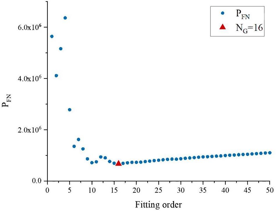
The penalty function PFN is used to measure the quality of the fit, by which it is possible to assess the effectiveness of the fit using different orders and select the fit order that minimizes the penalty function as the better-fit order NG.

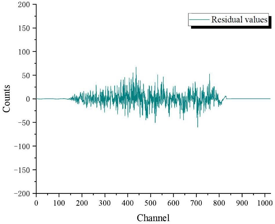
If the optimal fitting order NG does not yield satisfactory results, we can further consider the coefficient of determination R² (Eq. (10)) corresponding to the fitting function around NG. By evaluating the distribution of residual values in the ‘effective low-energy window’ for $i\in \left[n_{\text{low\_min}}\mathrm{,}{n}_{\text{low\_max}}\right]$ and the ‘effective high-energy window’ for $i\in \left[n_{\text{high\_min}}\mathrm{,}{n}_{\text{high\_max}}\right]$ regions as well as the smoothness of the curve after fitting, the optimal fitting order Nb can be determined as depicted in Fig. 5. SST (Eq. 11) represents the sum of the squares of the difference between the original data and its mean of the original data. Furthermore, SSR (Eq. 12) represents the sum of the squares of the difference between the fitted data and mean of the original data. C (Eq. 13) represents the average channel count. $R^2=\frac{SSR}{SST}=\frac{SST-S_N^2}{SST}=1-\frac{S_N^2}{SST}$ (10) $SST={\displaystyle \sum _{i=n_{\text{min}}}^{n_{\text{max}}}}{\left[C_i-\overline{C}\right]}^2$ (11) $SSR={\displaystyle \sum _{i=n_{\text{min}}}^{n_{\text{max}}}}{\left[f_F\left(i\right)-\overline{C}\right]}^2$ (12) $\overline{C}=\frac{1}{n_{\text{max}}-n_{\text{min}}}{\displaystyle \sum _{i=n_{\text{min}}}^{n_{\text{max}}}}{C}_i$ (13)

Fig. 5Full-screen View

Distribution of fitted differences

Once the order of the optimal fitting function Nb is determined, the hybrid logarithmic fitting energy spectrum can be plotted using (f_F(i)) points $i\in \left[n_{\text{min}}\mathrm{,}{n}_{\text{max}}\right]$. The ‘effective high energy window’ and ‘effective low energy window’ can then be set for the highest E_m nuclides in the current hybrid β-logarithmic fitting energy spectrum.

Cubic Spline Interpolation

The cubic spline interpolation function [33] ‘connects’ the 'effective low-energy window' and the ‘effective high-energy window’ of the hybrid β-logarithmic fitted energy spectrum to produce a smooth continuous curve, i.e., the highest E_m nuclide β-logarithmic fitting energy spectrum. It has the advantages of a simple formula, fast calculation speed, and good stability and is designed to ensure calculation efficiency by making the β-energy spectrum coherent, smooth, and retains the details of the original data in the entire energy range, which provides a more reliable and accurate basis for the subsequent analysis and interpretation of the data [34].

For y=f(x) in a given interval [a, b] with the given p nodes, $a=x_0<x_1<\dots <x_p<b$ and the function values $y_0\mathrm{,}{y}_1\mathrm{,}\dots \mathrm{,}{y}_p$ correspond to the p nodes. Furthermore, S(x) is termed as a cubic-spline interpolation function if it satisfies the following conditions:

1. On each subinterval $\left[x_{k-1}\mathrm{,}{x}_k\right]$ (k=1, 2, …, p), S(x) is a polynomial not higher than the third degree;

2. S(x) is 2nd order derivable in [a, b] interval and the derivative function is continuous, i.e., $S(x)\in C^2\left[a\mathrm{,}b\right]$;

3. The function S(x_k) is equal to the function value yk (k=1, 2, ..., n).

From condition (1), S(x) in each $\left[x_{k-1}\mathrm{,}{x}_k\right]$ interval can be expressed as Eq. (14): $S\left(x_k\right)=a_k+b_{k}x+c_k{x}^2+d_k{x}^3\left(k=\mathrm{1,}\mathrm{2,}\dots \mathrm{,}p\right)$ (14) To determine the interpolation function in p intervals, 4p conditions are required for the 4p coefficients to be determined {ak}, {bk}, {ck}, {dk}. From Condition (2), S(x) should satisfy the conditions shown in Eq. (15) at each node xk and 3p-3. $\{\begin{array}{ll}{S}^{-}\left(x_k\right)=S^{+}\left(x_k\right)\hfill & \hfill \\ {S^{\prime }}^{-}\left(x_k\right)={S^{\prime }}^{+}\left(x_k\right)\hfill & (k=\mathrm{1,}\mathrm{2,}\mathrm{3,}\dots \mathrm{,}p-1)\hfill \\ {S^{″}}^{-}\left(x_k\right)={S^{″}}^{+}\left(x_k\right)\hfill & \hfill \end{array}$ (15) From condition (3) above, S(x) must satisfy all p+1 conditions shown in Eq. (16), and there are already 4p-2 conditions in the above statistics. $S\left(x_k\right)=y_k(k=\mathrm{0,}\mathrm{1,}\mathrm{2,}\mathrm{3,}\dots \mathrm{,}p)$ (16) Finally, by adding two boundary conditions, 4p coefficients and S(x_k) can be determined: The following three boundary conditions are commonly used.

1. Given the values of the first order derivatives at the two endpoints: $\{\begin{array}{l}{S}^{\prime }\left(x_0\right)=z_0\hfill \\ S^{\prime }\left(x_p\right)=z_p\hfill \end{array}$ (17) 2. Given the values of the second order derivatives at the two endpoints, where it becomes a natural boundary condition when $z_0=z_p=0$: $\{\begin{array}{l}{S}^{″}\left(x_0\right)=z_0\hfill \\ S^{″}\left(x_p\right)=z_p\hfill \end{array}$ (18) $\{\begin{array}{l}{S}^{″}\left(x_0\right)=z_0=0\hfill \\ S^{″}\left(x_p\right)=z_p=0\hfill \end{array}$ (19) 3. S(x) is a function with period b-a: $\{\begin{array}{l}{S}^{-}\left(x_0\right)=S^{+}\left(x_p\right)\hfill \\ {S^{\prime }}^{-}\left(x_0\right)={S^{\prime }}^{+}\left(x_p\right)\hfill \\ {S^{″}}^{-}\left(x_0\right)={S^{″}}^{+}\left(x_p\right)\hfill \end{array}$ (20) Specifically, to ‘connect’ the ‘effective low-energy window’ and the ‘effective high-energy window’ using cubic spline interpolation functions, we utilize the fitted spectrum line f_F(x)=y with a given set of p nodes $x_0<x_1<\dots <x_p$ and corresponding function values $y_0\mathrm{,}{y}_1\mathrm{,}\dots \mathrm{,}{y}_p$ as interpolation points within the interval $x\in \left[n_{\text{low\_min}}\mathrm{,}{n}_{\text{low\_max}}\right]\cup \left[n_{\text{high\_min}}\mathrm{,}{n}_{\text{high\_max}}\right]$ [35-37]. This was conducted to perform a cubic spline interpolation. To ensure smoothness and low-count properties at high- and low-energy ends of the hybrid logarithmic fitted energy spectrum, the first-order derivatives, as shown in Eq. (21), are used as boundary conditions in the calculation of the cubic spline interpolation function [38, 39]. $\{\begin{array}{l}{S}^{\prime }\left(x_0\right)=0\hfill \\ S^{\prime }\left(x_p\right)=0\hfill \end{array}$ (21) By employing cubic spline interpolation to derive the logarithmic fitting energy spectrum of the highest E_m nuclide in the hybrid logarithmic fitting energy spectrum, the current hybrid logarithmic fitting energy spectrum is subtracted from the logarithmic fitting energy spectrum to yield a logarithmic fitting energy spectrum comprising the remaining lower E_m nuclides. Subsequently, new ‘effective low-energy window’ and ‘effective high-energy window’ selections are made in this energy spectrum and inputted into the interpolation analysis process. Iterating through this process allows the resolution of the logarithmic energy spectrum of each nuclide in the original hybrid logarithmic energy spectrum. Finally, activity calculations were performed for each resolved log-fit energy spectrum.

Algorithmic Process

This algorithm has five main modules: logarithmic conversion, curve fitting, cubic spline interpolation processing, difference processing, and activity calculation. The specific process is as follows.

1. Use the logarithmic processing function provided by the liquid scintillation spectrometer to convert the β-linear energy spectrum into a logarithmic energy spectrum;

2. Curve fitting of the hybrid logarithmic energy spectrum using an ‘optimized’ Fourier series function model with ‘effective high energy windows’ and ‘effective low energy windows’ for the highest E_m nuclides in the current hybrid β-logarithmic fitted energy spectrum;

3. Select the ‘effective high-energy window’ and ‘effective low-energy window’ in the hybrid β log-fit energy spectrum and use cubic spline interpolation to obtain the log-fit energy spectrum of the β nuclide with the highest E_m;

4. Differencing the current hybrid log-fit energy spectrum with the log-fit energy spectrum of the β-nuclide with the highest E_m yields a new hybrid log-fit energy spectrum comprising the other β-nuclides with lower E_m. Substituting this into Step 3 and iterating according to the previous procedure, the logarithmic energy spectrum of each nuclide can be resolved;

5. After resolving the hybrid logarithmic energy spectrum, an activity calculation is performed for each of the resolved logarithmic fitted energy spectra. The activity calculation formula is shown in Equation 22. Here, A denotes the source activity, C denotes the total counts of the energy spectrum, t denotes measurement time, ε denotes detection efficiency, and R denotes sample recovery rate. $A=\frac{C}{t\epsilon R}$ (22)

GEANT4 Simulation of ¹⁴C⁹⁰Sr⁹⁰Y Energy Spectrum Analysis

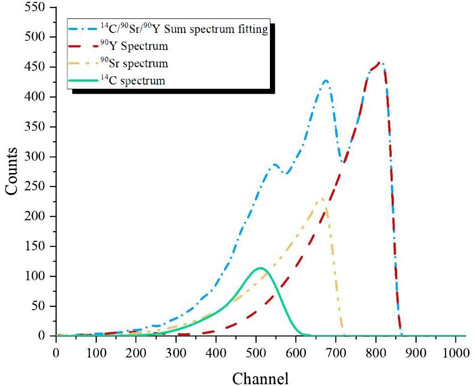
The GEANT4 simulated ¹⁴C/⁹⁰Sr/⁹⁰Y hybrid logarithmic fitted energy spectrum shown in Fig. 6 is fitted using an ‘optimized’ Fourier series function model. Considering that E_m = 0.156 MeV for ¹⁴C, 0.546 MeV for ⁹⁰Sr, and 2.284 MeV for ⁹⁰Y, the part of the channel group at the high-energy end of the energy interval from 0.546 MeV to 2.2839 MeV (750 to 870 channel group) and the ‘presence’ section after the zero channel are all counted. Part of the low-energy end of the channel group (channels 0–140), where the counts are all zero, can be considered to be contributed by ⁹⁰Y with the highest E_m in the mixing spectrum alone. Therefore, the 750 to 870 channel groups and the 0 to 140 channel groups of the fitted spectra are selected as the ‘effective high-energy window’ and ‘effective low-energy window’ corresponding to the highest E_m nuclide ⁹⁰Y and then they are ‘connected’ using cubic spline interpolation. Then, using the cubic spline interpolation process, we ‘connect’ them to obtain a smooth spectrum, i.e., the β-logarithmic fitted spectrum corresponding to the ⁹⁰Y nuclide.

Fig. 6Full-screen View

(color online) ¹⁴C/⁹⁰Sr/⁹⁰Y hybrid β-logarithmic fitted energy spectrum

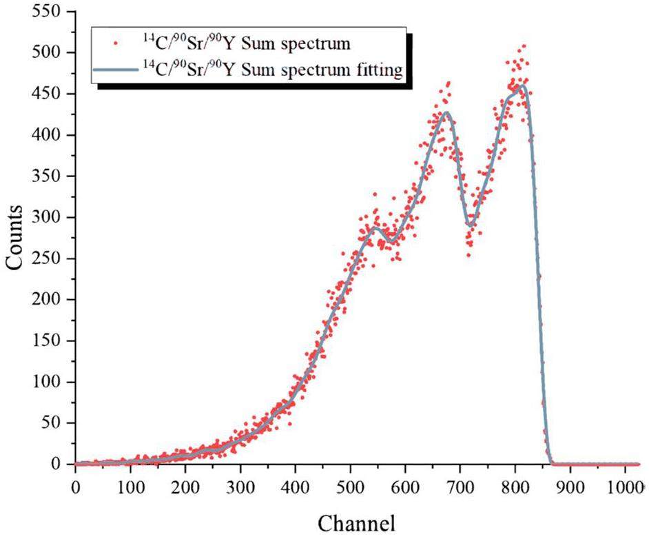
In the order of E_m from largest to smallest (⁹⁰Y → ⁹⁰Sr → ¹⁴C), the ¹⁴C/⁹⁰Sr/⁹⁰Y hybrid log-fit energy spectrum is initially processed by difference with the log-fit energy spectrum of ⁹⁰Y to obtain the ¹⁴C/⁹⁰Sr hybrid log-fit energy spectrum. Subsequently, ¹⁴C/⁹⁰Sr hybrid log-fit energy spectrum is processed using cubic spline interpolation to obtain a log-fit energy spectrum corresponding to the ⁹⁰Sr nuclide. Next, the ¹⁴C/⁹⁰Sr hybrid log-fit energy spectrum is processed based on the difference from the log-fit energy spectrum of ⁹⁰Sr to obtain the ¹⁴C log-fit energy spectrum. Finally, ¹⁴C/⁹⁰Sr/⁹⁰Y log-fit energy spectrum and the resolved ¹⁴C, ⁹⁰Sr, and ⁹⁰Y log-fit energy spectra were obtained as shown in Fig. 7.

Fig. 7Full-screen View

(color online) Spectrogram for ¹⁴C/⁹⁰Sr/⁹⁰Y

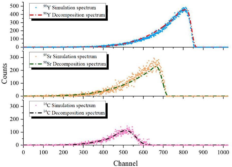
Based on the presentation in Fig. 8, we compared ¹⁴C, ⁹⁰Sr, and ⁹⁰Y energy spectra, which is obtained by using the Fourier fitting interpolation method with the original GEANT4 simulated energy spectra. The results showed good agreement between the two methods, verifying the feasibility and validity of the Fourier fitting interpolation method in the experimental setting of a liquid scintillation spectrometer. This shows that the energy spectra obtained by the Fourier fitting interpolation method are consistent with the actual simulation data and can accurately reflect the distribution of the particle energy spectra under experimental conditions. This result provides strong support for the use of Fourier fitting interpolation for liquid scintillation spectrometer data analysis and provides a reliable method and basis for the further development of liquid scintillation spectrometers in nuclear physics experiments and applications.

Fig. 8Full-screen View

(color online) Comparison of ¹⁴C/⁹⁰Sr/⁹⁰Y logarithmic fitted energy spectral analysis effects

Activity Error Analysis

3.2.1

Fourier Fitting Interpolation Method

To measure the ⁹⁰Sr/⁹⁰Y sample source, the liquid scintillation spectrometer used was the Quantulus1220 ultra-low background liquid scintillation spectrometer from Perkin Elmer, USA. The detection efficiencies for ³H and ¹⁴C were 25% and 68%, respectively. The background counting rate (relative to the ³H energy region) was 0.067 s^-1. The distance between the source and scintillator incident window was set to 1 mm, and the measurement time was 7200 s. The Fourier-fitting interpolation method was used to analyze the energy spectrum of the ⁹⁰Sr/⁹⁰Y sample source. The results show that the measured detection efficiency of the liquid scintillation spectrometer for the ⁹⁰Sr/⁹⁰Y sample source was 25.721%. The full-spectrum detection efficiency of GEANT4 simulation was 27.24%. Given that the initial activity of the ⁹⁰Sr/⁹⁰Y sample source is 371.44 Bq and the half-life of ⁹⁰Y is 64 h, it can be concluded that ⁹⁰Sr and ⁹⁰Y in the sample are in a long-term equilibrium state. Therefore, the activities of ⁹⁰Sr and ⁹⁰Y are equal, indicating that the actual activity of ⁹⁰Y is 185.72 Bq.

According to the process described above, the 35th-order ‘optimized’ Fourier series function is used to fit the measured energy spectrum of ⁹⁰Sr/⁹⁰Y and channel group of 340 to 500 is selected as the ‘effective high-energy window’ corresponding to ⁹⁰Y. By analyzing the Geant4 simulation results and liquid scintillation energy spectrum data, the corresponding channel of 23.8 keV in the logarithmic energy spectrum of ⁹⁰Sr/⁹⁰Y was still in the channel group with a count of zero, and a channel group of 1 to 10 was selected as the ‘effective low-energy window’ of ⁹⁰Y. Using cubic spline interpolation to ‘connect’ the ‘effective high-energy window’ and the ‘effective low-energy window’ to get a smooth spectrum, i.e., the ⁹⁰Y energy spectrum. The fitted ⁹⁰Sr/⁹⁰Y energy spectrum is subtracted from ⁹⁰Y energy spectrum to obtain the ⁹⁰Sr energy spectrum. The results of the Fourier-fitting interpolation method for the ⁹⁰Sr/⁹⁰Y sample source are shown in Fig. 9.

Fig. 9Full-screen View

(color online) Results of Fourier fitting interpolation analysis of the measured spectra of ⁹⁰Sr/⁹⁰Y sample source

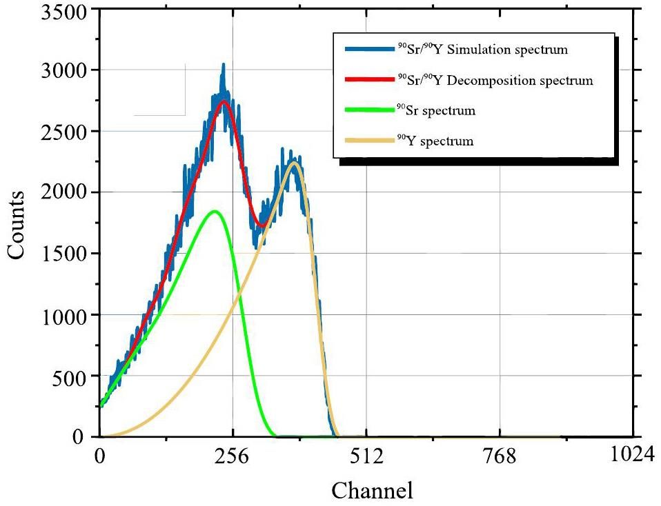
By analyzing the results of the Fourier fitting interpolation method, we obtain the following conclusions: the average count rate per minute of ⁹⁰Y is 3173.803 CPM, i.e., the activity of ⁹⁰Y corresponding to 25.721% of the measured detection efficiency is 205.66 Bq with a relative error of 10.737%; similarly, the activity of ⁹⁰Y corresponding to 27.24% of the simulated full-spectrum detection efficiency is 194.20 Bq with a relative error of 4.568%. These results are consistent with the test expectations and show that the Fourier fitting interpolation method has a high accuracy and reliability when analyzing the experimental data. These analytical results provide an important reference for the further study and application of the performance of ⁹⁰Y in liquid scintillation spectrometers, as well as an experimental basis for the optimization and improvement of liquid scintillation spectrometers.

3.2.2

Asym2Sig Method

First, an asymmetric double sigmoid function is used to fit the measured logarithmic energy spectrum data of a pure ⁹⁰Y sample source. The initial values of the fitting parameters (w₁, w₂, w₃) in the A-term asymmetric double-sigmoid function are determined as 109.9, 74.75, and 12.92, respectively. Based on ⁹⁰Sr/⁹⁰Y sample source β, set the peak count channel locations corresponding to ⁹⁰Y and ⁹⁰Sr in the logarithmic energy spectrum and set the initial fitting parameters of the shape parameters (x_c, x_b) to 350 and 180. The asymmetric double-sigmoid function can be obtained as Eq. (24): $\begin{array}{l}\delta =\frac{1}{1+e^{-\left(x-x_c+\frac{w_1}{2}\right)/w_2}}\mathrm{,}\\ \eta =\frac{1}{1+e^{-\left(x-x_c-\frac{w_1}{2}\right)/w_3}}\mathrm{,}\\ \theta =\frac{1}{1+e^{-\left(x-x_b+\frac{w_{b1}}{2}\right)/w_{b2}}}\mathrm{,}\\ \kappa =\frac{1}{1+e^{-\left(x-x_b-\frac{w_{b1}}{2}\right)/w_{b3}}}\end{array}$ (23) $\begin{array}{l}y(x)=A\cdot \left(\delta \cdot (1-\eta )\right)+B\cdot \left(\theta \cdot (1-\kappa )\right)\hfill \end{array}$ (24) On this basis, the sum of the asymmetric double sigmoid functions A and B is used to evaluate ⁹⁰Sr/⁹⁰Y β, perform curve fitting on the logarithmic energy spectrum, and determine the final fitted values of 10 shape parameters (A, x_c, w₁, w₂, w₃) and (B, x_b, w_b1, w_b2, w_b3) as 3054, 347.8, 110.9, 74.35, 12.92, and 2503, 182.1, 143.8, 56.98, 14.5. Finally, the ten determined shape parameters (A, x_c, w₁, w₂, w₃) and (B, x_b, w_b1, w_b2, w_b3) were fed into the single asymmetric double-sigmoid function to obtain the logarithmic energy spectra of ⁹⁰Sr and ⁹⁰Y. The energy-spectrum analysis results of the Asym2Sig method for the ⁹⁰Sr/⁹⁰Y sample source are shown in Fig. 10.

Fig. 10Full-screen View

(color online) Analysis results of Asym2Sig method for the measured spectrum of ⁹⁰Sr/⁹⁰Y sample source

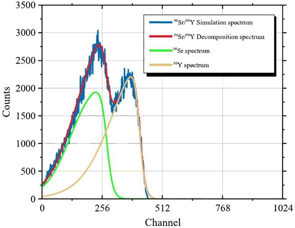
The analysis results of the Asym2Sig method show that the average count rate per minute for ⁹⁰Y is 3154.871 CPM, which corresponds to 25.721%. The actual detection efficiency and activity of ⁹⁰Y are 204.434 Bq with a relative error of 10.077% and ⁹⁰Y, which corresponds to a simulated full-spectrum detection efficiency of 27.24% with an activity of 193.029 Bq and a relative error of 3.936%, which satisfied the testing expectations.

In summary, the logarithmic energy spectrum analysis results of the measured ⁹⁰Sr/⁹⁰Y sample source using the Asym2Sig and Fourier fitting interpolation methods show that ⁹⁰Y activity errors analyzed by the two spectral-solving algorithms using the actual detection efficiency are both approximately 10%. When using the simulated full-spectrum detection efficiency, the errors are all within 5%, which is in line with experimental expectations. Moreover, the relative error of ⁹⁰Y activity analyzed using the Asym2Sig method is smaller than that of the Fourier fitting interpolation method, indicating better analysis results. However, given the need to detect pure ⁹⁰Y sample sources in advance, the analysis using the Asym2Sig method is more cumbersome than that using the Fourier fitting interpolation method. In the actual analysis process, the above two energy spectrum analysis methods can be selected based on the on-site experimental conditions.